1. INTRODUCTION

This paper presents a new test statistic for comparing two means μ1 and μ2 under the following two types of data:

1. Type U Data: Data obtained from two independent random samples but, unknowingly or by accident, some units are used or found to be the same in both samples that resulted in some paired observations. The number of units common to both samples is expected to be small compared to unpaired sample sizes.

2. Type P Data: Data obtained from paired design, but some data values are missing completely at random that resulted in some unpaired observations. Pairs with both missing observations are deleted. The numbers of first and second missing values (or equivalently the unpaired sample sizes) are expected to be small compared to complete pairs.

Type U data may be visualized as two random samples (X1,U1)=x11,x12,…,x1n1,u11,u12,…,u1n, and (X2,U2)=x21,x22,…,x2n2,u21,u22,…,u2n of which (U1,U2)=(u11,u21), (u12,u22),…, (u1n,u2n) are paired, and X1=x11,x12,…,x1n1 and X2=x21,x22,…,x2n2 are unpaired observations of the two independent samples.

Type P data is visualized as n1+n2+n pairs (X1,.), (.,X2),(U1,U2) where n1 pairs (X1,.) have only second observations missing, n2 pairs (.,X2) pairs have only first observations missing, and n complete pairs (U1,U2) with no missing observations.

We assume that the paired data (U1,U2) is a random sample from a bivariate normal distribution BN(μ1,μ2,σ12,σ22,ρ), and the unpaired data X1 and X2 are independent random samples from normal distributions N(μ1,σ12) and N(μ2,σ22), respectively. Notice that the means and variance parameters are same in bivariate normal and normal distributions.

Some studies that require testing H0:μ1−μ2=0 for Type U and Type P data described above are mentioned by several researchers (e.g., Uddin and Hasan [1], Samawi and Vogel [2], Rempala and Looney [3], Mehrotra [4], Looney and Jones [5], Hermann and Looney [6], Dimery et al. [7], Steere et al. [8], Nurnberger et al. [9], Bhoj [10], Ekbohm [11], Lin and Stivers [12]). A survey of various statistical methods proposed for use in this setting can be found in Guo and Yuan [13].

If the number (n) of paired data is too small compared to unpaired sample sizes n1 and n2, one may simply ignore the paired data and use two independent samples methods (e.g., independent samples t-test). Similarly, paired sample methods (e.g., paired t-test) can be used if the unpaired sample sizes n1 and n2 are too small compared to n, the complete pairs. A third approach would be to ignore the pairing of data and run the two independent samples t-test. In each of the above three approaches, some information would be lost due to omitted observations or correlations between paired observations.

The present paper focuses only on tests of H0:μ1−μ2=0 that use all available data on both samples as well as the correlation from paired observations. For the purpose of a brief literature review, first we use the following notations:

• x¯i = sample mean of ni observations xi1,xi2,…,xini, i=1,2.

• sii2 = sample variance of ni observations xi1,xi2,…,xini, i=1,2.

• Mi = sample mean of ni+n observations xi1,xi2,…,xini,ui1,ui2,…,uin, i=1,2.

• si2 = sample variance of ni+n observations xi1,xi2,…,xini,ui1,ui2,…,uin, i=1,2.

• d¯ = sample mean of n paired differences u1j−u2j,j=1,2,…,n.

• sd2 = sample variance of n paired differences u1j−u2j,j=1,2,…,n.

• sd∗2 = sample variance of n weighted paired differences nu1j∕(n1+n)−nu2j∕(n2+n), j=1,2,…,n.

For Type U data under the assumption that σ12=σ22, Bhoj [10] suggested the following test statistic Tc:

The above test statistic Tc is linear combination of the two independent samples t-statistic tfe for unpaired data with fe=n1+n2−2 degrees of freedom and paired t-test statistic tfp with fp=n−1 degrees of freedom. To accommodate for unequal variances, Tc is modified by Uddin and Hasan [1] to Tcu:

The sampling distribution of tfu is approximated by t-distribution with Satterthwaites [14] approximate degrees of freedom fu, where

Looney and Jones [5] proposed the following alternative to Tc:

However, it is pointed out by Uddin and Hasan [1] that the test statistic Zcorr has a negative estimated variance problem and offered a solution to the problem. They suggest to modify Zcorr to Zc as follows:

For the Type P data that results from a paired design with missing observations, Mehrotra [4] suggested that a test (here referred to as REML) of the above hypothesis can be carried out using SAS Proc Mixed.

The above test statistics are empirically compared with respect to type I error rates and powers for some selected values of sample sizes and correlations (see Uddin and Hasan [1], Mehrotra [4]). Under the assumption of equal variances, Mehrotra [4] used simulations to compare type I error rates and powers of REML, Zcorr and Tc and concluded that REML results in higher power than both Tc and Zcorr for large positive correlations.

In a recent paper, Uddin and Hasan [1] modified Zcorr to Zc to correct for negative estimated variance problem, Tc to Tcu to account for unequal variances, and carried out a simulation study to compare REML, Zc and Tcu. For normally distributed data with equal variances, their simulation results provided empirical support to conclude that REML results in higher powers than Zc and Tcu for large positive correlations. For all negative and small to moderate positive values of correlation, Zc appears to have higher powers than both REML and Tcu. For samples from normal distributions with unequal variances, Zc is outperformed jointly by Tcu and REML, where REML is preferred to Tcu for large positive correlations (ρ) and Tcu for all other correlations. The choice of a test statistic thus depends on ρ which will often be unknown in practice. Viewing this as a limitation of the above approaches, this paper is devoted to finding a single test statistic that would outperform others for all ρ with respect to statistical powers while keeping the type I error rates very competitive.

In Section 2 below, we describe such a test statistic and offer approximate null sampling distribution of the proposed test statistic. Following an example in Section 3 from Rempala and Looney [3], we use simulation to show that the proposed test statistic performs very well in comparison to the alternative methods available in the literature for samples from normal and logistic distributions with equal variances.

2. PROPOSED TEST STATISTIC AND APPROXIMATE NULL SAMPLING DISTRIBUTION

As noted above both Tc and Tcu are defined as weighted average of unpaired and paired t-statistic. An alternative test statistic considered here is based on the weighted average L(ω)=ω(x¯1−x¯2)+(1−ω)(u¯1−u¯2) of unpaired and paired mean differences with ω∈(0,1) chosen so that var(L(ω))=ω2σ(x¯1−x¯2)2+(1−ω)2σd¯2 is minimized. It follows that ω=σd¯2σ(x¯1−x¯2)2+σd¯2 minimizes this variance where σd¯2 is the variance of the sampling distribution of paired mean difference d¯ and σ(x¯1−x¯2)2 is the variance of the sampling distribution of (x¯1−x¯2). If the null hypothesis H0 is true and variances are known, then

is distributed as standard normal. In practice, the variances σ(x¯1−x¯2)2 and σd¯2 and hence ω will be unknown and must be estimated from data. Since σ(x¯1−x¯2)2 is the variance of the sampling distribution of (x¯1−x¯2), a function of only unpaired observations, it is sensible to estimate this variance from unpaired data only. Similarly, σd¯2 can be estimated using paired observations only. Analogous to paired and independent samples test of H0:μ1=μ2, we suggest the following estimators:

Replacing the unknown variances and hence ω by their estimates as shown above, and using a correction factor for the purpose of sampling distribution, we define the following test statistic:

It is noted here that the above Tu without the correction factor θ reduces to TNew of Samawi and Vogel [2] when ω̂=1∕2 and the common variance σ12=σ22=σ2 is estimated by the pooled variance of the unpaired samples. Here, we do not know the exact sampling distribution of Tu under the null hypothesis. Following the procedure described in Uddin and Hasan [1], we approximate the null sampling distribution of Tu by t-distribution with (4D−6C2)∕(D−3C2) degrees of freedom. This approximate null distribution is used in our simulation in Section 4 for the calculation of empirical type I error rates and powers of Tu for some selected values of sample sizes and correlation values of paired observations. We have an illustrative example in Section 3 below.

3. A NUMERICAL EXAMPLE

In this example, we use the data from a clinical study on symptom management among hospice patients in the last days of life (see Hermann and Looney [6], Rempala and Looney [3]). The data values reported in Table 3 of Rempala and Looney [3] are Karnofsky Performance Status (KPS) scale scores. These values are obtained from 37 patients on the day before they died, from 32 patients on their last day of life, but nine patients were common on both days. The reader may review Hermann and Looney [6], Rempala and Looney [3] for more details of this clinical study on symptom management among hospice patients in the last days of life. This study results in data in the above setting with unpaired samples of sizes n1=28, n2=23 and n=9 paired (next-to-last day, last day) data values (see Table 3 in Rempala and Looney [3] for all data values). Summary results obtained from these samples are reported by Uddin and Hasan [1] in their Table 1. These samples yield Tu=2.83 with 16.01 degrees of freedom and two-sided p-value =0.012 which is small enough to conclude that the KPS mean ratings on the last day and next-to-last day of life are significantly different. This conclusion is consistent with that reported by Uddin and Hasan [1] in their Table 2 under five other test statistics considered in that paper. An R program is displayed in Table 1 that can be used to do the calculations where the user needs only to enter the data and run the program.

4. SIMULATION: DISTRIBUTIONS AND PARAMETERS

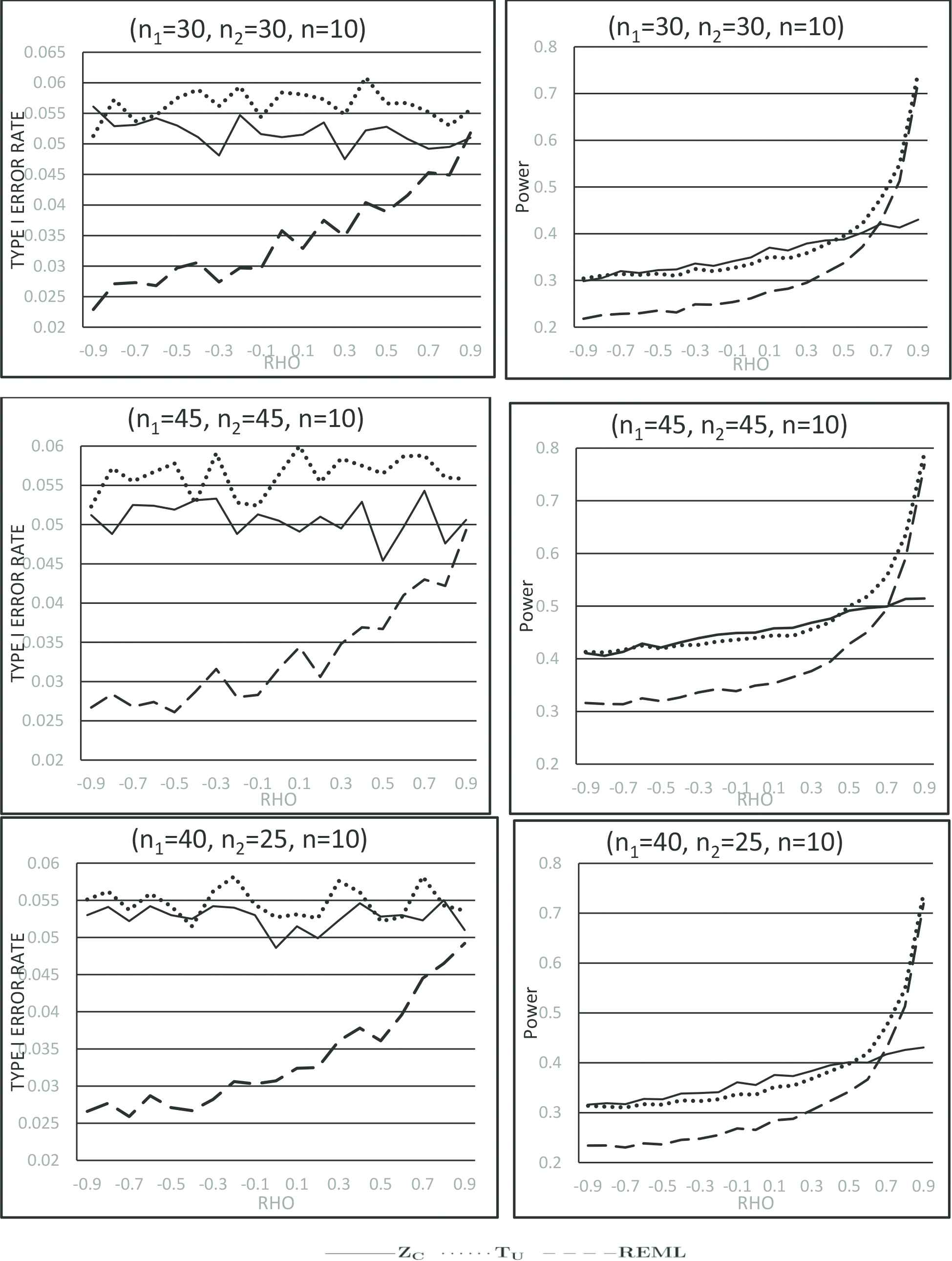
To make it comparable to other simulation studies reported in the literature (e.g., Uddin and Hasan [1], Mehrotra [4]), we set our null and research hypothesis as H0:μ1−μ2=0 and H1:μ1−μ2=0.35 respectively. For some sample sizes and correlations, 10,000 random samples are generated from the corresponding normal and bivariate normal distributions with σ12=σ22=1 under both null and research hypothesis. SAS IML (version 9.22) functions “rand(‘normal’, μ, σ)” and “randnormal(n, mean, cov)” are used for generating these samples. For each set of simulation parameters, type I error rates when H0:μ1−μ2=0 and powers when H0:μ1−μ2=0.35 were calculated for each of Zc, REML and Tu based on 10,000 samples mentioned above. Note that Tcu is not included here in our simulation with sampling from normal distributions with equal variances since Zc and REML are found by Uddin and Hasan [1] to jointly outperform Tcu for all correlation values. Our goal here is to compare the proposed test statistic Tu to Zc and REML with respect to type I error rate and power. In the calculation of type I error rates and powers, we have used the null sampling distribution of Tu from Section 2 above, but for Zc, the null distribution described in Uddin and Hasan [1] is used. However, for REML, both type I error rate and power are determined by comparing significance probabilities obtained from the analysis carried out by SAS Proc Mixed with nominal α=0.05. The empirical type I error rates and powers obtained from our simulations are presented graphically in Figures 1 and 2 for some combinations of sample sizes and parameter values.

Figure 1

Type I error rates and powers for samples from normal distributions with equal variance.

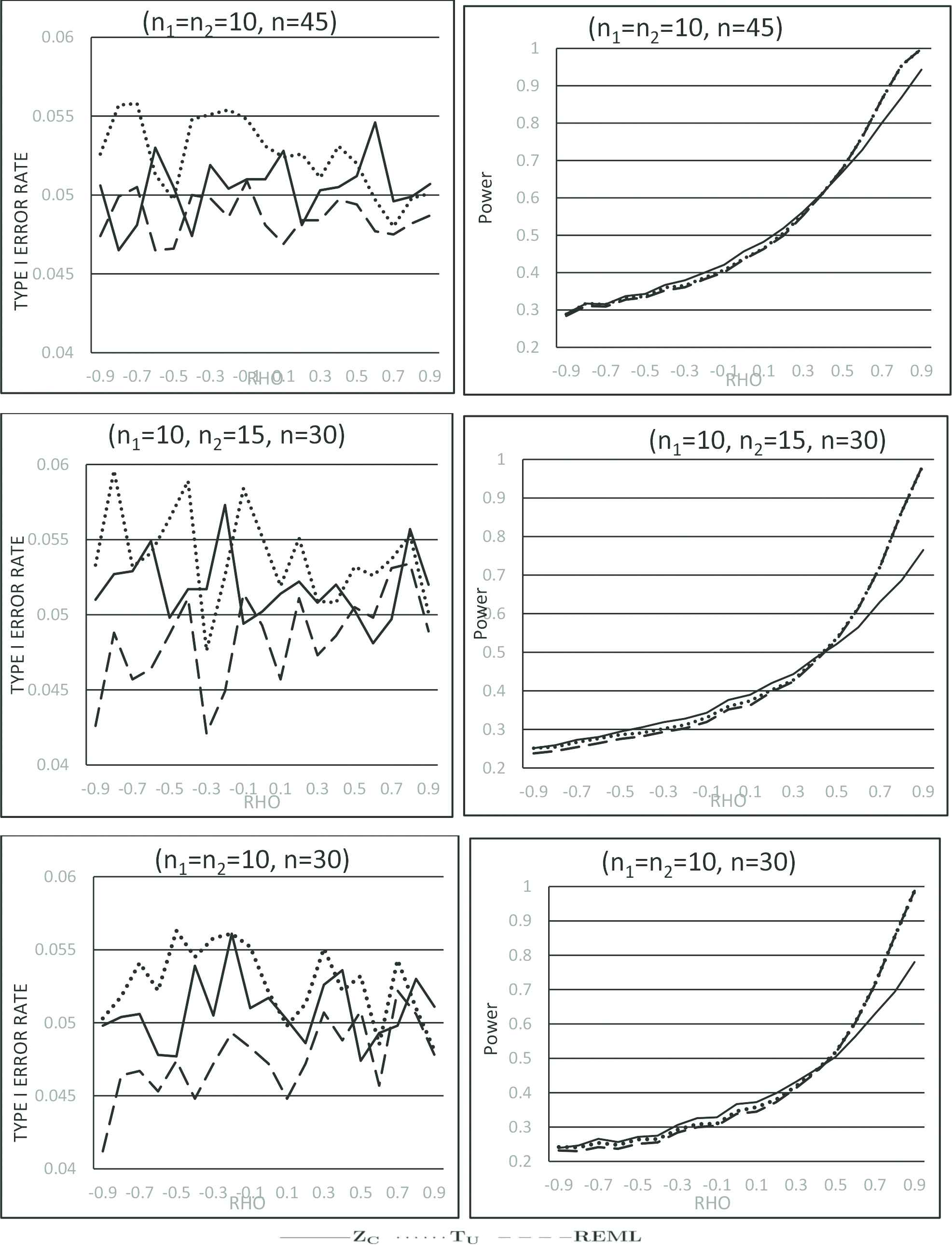
Figure 2

Type I error rates and powers for samples from normal distributions with equal variance.

To study the robustness of the proposed test statistic, the above simulation is repeated for samples from logistic distribution, a non-normal symmetric distribution similar to normal but with heavier tails than the normal. The i-th logistic probability density function is given by

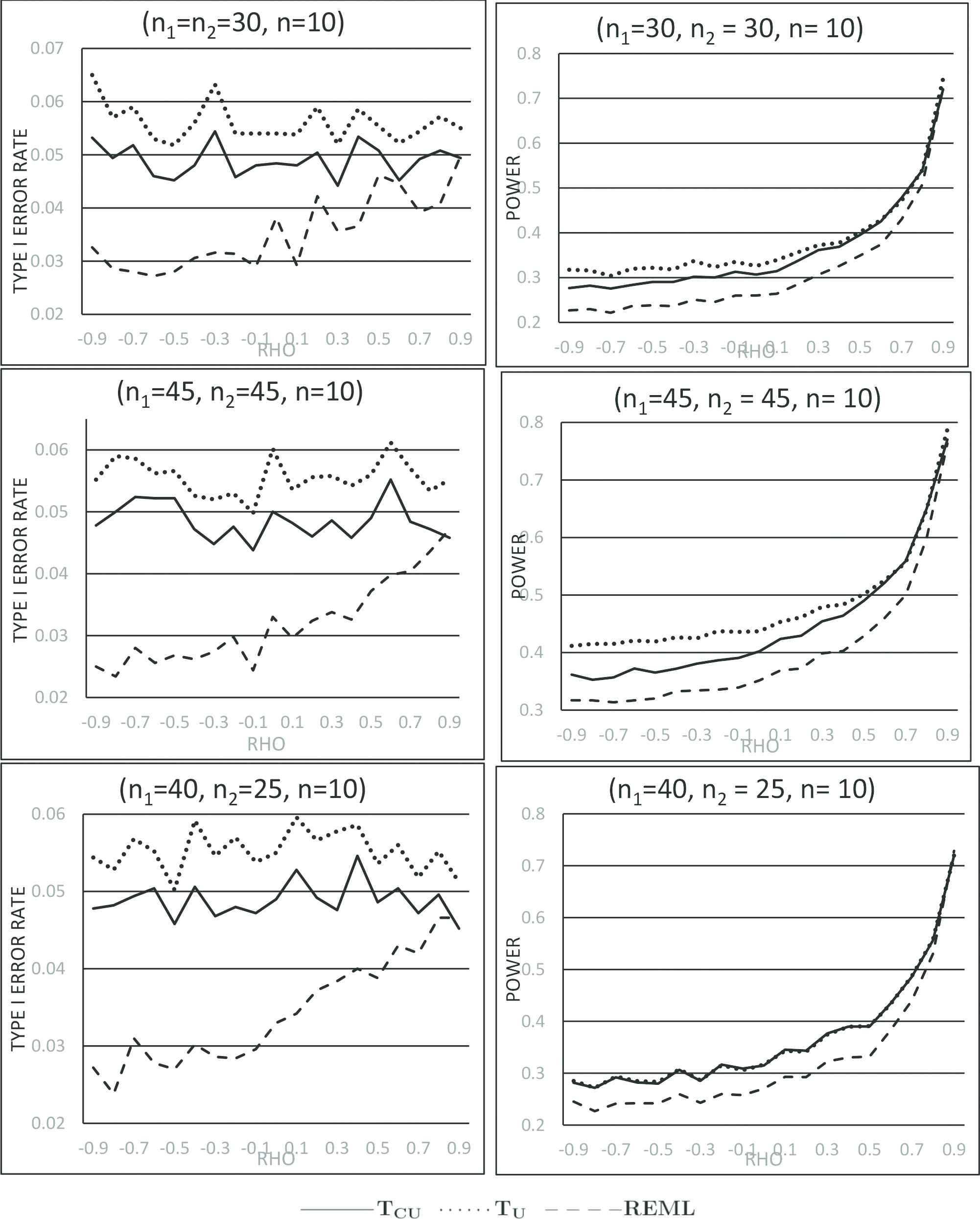
for which the mean and variance are μi and σi2π2∕3. For notational convenience, we shall use μiℓ and σiℓ2 to refer to the mean and variance of the i-th logistic distribution, i=1,2. The null and research hypotheses are set as H0:μ1ℓ−μ2ℓ=0, H1:μ1ℓ−μ2ℓ=0.35, and standard deviations of the two distributions are set at (σ1ℓ,σ2ℓ) = (1, 1). Since the bivariate logistic distribution with the above marginal logistic distributions yield only ρ=1∕2, we randomly generated correlated pairs of cumulative probabilities, and then utilize the cumulative distribution function of the above logistic distribution to generate the paired sample data. This technique was previously used by Uddin and Hasan [1] in their simulation. Using samples from logistic distributions, Uddin and Hasan [1] provided empirical support in favor of using REML or Zc depending on sample sizes and correlation values. Here the empirical type I error rates and powers of the proposed test statistic Tu, displayed in Figures 3 and 4, are compared to that of REML and Zc using samples from logistic distributions described above.

Figure 3

Type I error rates and powers for samples from logistic distributions with equal variance.

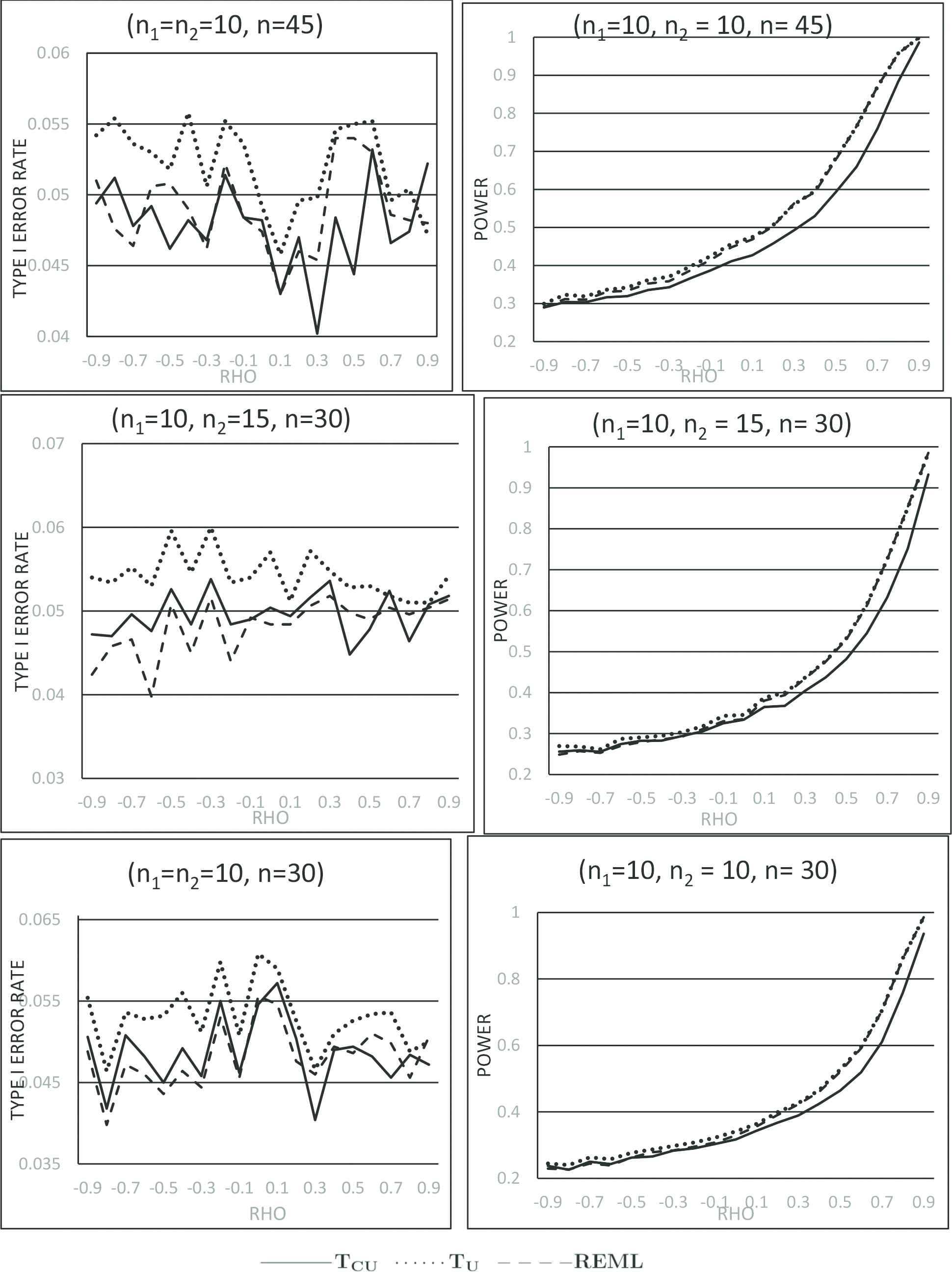
Figure 4

Type I error rates and powers for samples from logistic distributions with equal variance.

5. DISCUSSION AND CONCLUSION

For sampling from normal distributions with equal variances, the test statistic Tu shows higher power than REML for all ρ, and higher powers than Zc for moderate to large ρ considered here. However, due to the higher type I error rates of Tu, particularly for negative ρ and type U data (see Figure 1) compared to that of Zc and REML, one may argue that such power gains by Tu over Zc and REML is the result of its inflated type I error rates. However, for type P data with positive ρ (see Figure 2), the competitive empirical type I error rates and power curves provide empirical support in favor of recommending Tu over Zc and REML. Note that for type P data, we expect small unpaired sample sizes n1, n2 compared to paired sample size n whereas for type U data only a small number of complete pairs is expected compared to unpaired sample sizes. Note further that the correlation parameter ρ is expected to be positive in practice for paired data.

To investigate the robustness of Tu to non-normal distributions, we repeated our simulation using samples from logistic distributions described above. The test statistic Zc was found by Uddin and Hasan [1] to be more liberal with respect to type I error rates in the sense that Zc results in higher empirical type I error rates than the nominal α value. They argued in favor of choosing Tcu or REML depending on sample sizes and correlations for comparing means of logistic distributions. We thus excluded Zc and compared the proposed Tu with Tcu and REML. The empirical type I error rates and powers of Tu, REML, and Tcu are displayed in Figures 3 and 4. A closer look at the plots in these two figures reveal that Tcu results in higher type I error rate than the nominal α whereas REML is more conservative with smaller type I error rate than the assumed nominal α value for type U data. However, for type P data with positive correlations, the three test statistics appear to be very competitive with respect to type I error rates and Tu performs better with respect to power.

The present simulation study thus provided empirical support for choosing Tu for testing the equality of two means for type P data from normal distributions as well as from logistic distributions with equal variances when correlations of paired observations are positive. This is in contrast to findings in other simulations where, in the absence of Tu, the choice of a test statistic depends on paired/unpaired sample sizes and correlations of paired data.

We have expanded our simulation to investigate the robustness of Tu for unequal variances for all sample sizes and correlations shown in Figures 1–4 for both normal and logistic distribution. We followed the same procedure described in Uddin and Hasan [1] for these expanded simulations. The proposed statistic Tu does not appear to perform well when compared to others when variances are unequal. We like to note that the empirical comparisons of these methods are limited in that the simulations are carried out only for some selected combinations of n1,n2, n, σ1,σ2, and ρ with H1:μ1−μ2=0.35 using samples from normal and logistic distributions.

CONFLICT OF INTEREST

There is no conflict of interest.

AUTHORS' CONTRIBUTIONS

The two authors contributed equally to prepare this paper for publication.

Funding Statement

The work was not funded by any funding agency.

ACKNOWLEDGMENTS

The authors thank the Editor for carefully reading the manuscript and for his guidance on format in preparing this final version of the paper.