
Exponentiated Power Function Distribution: Properties and Applications
 , Muhammad Zafar Iqbal2, , Munir Ahmad1
- DOI
- 10.2991/jsta.d.200514.001How to use a DOI?
- Keywords
- Exponentiated distribution; Power function distribution; Bathtub-shaped failure rate; Order statistics; Rényi entropy; Maximum likelihood estimation
- Abstract
In this study, we have focused to propose a flexible model that demonstrates increasing, decreasing and upside-down bathtub-shaped density and failure rate functions. The proposed model refers to as the exponentiated power function (EPF) distribution. Some mathematical and reliability measures are developed and derived. We develop explicit expressions for the moments, quantile function and order statistics. Some shapes of the density and the reliability functions are sketched out and discussed. We suggest the method to estimate the unknown parameters of EPF by the maximum likelihood estimation. Two suitable lifetime datasets from engineering sector are used to explore the dominance of the EPF distribution.
- Copyright
- © 2020 The Authors. Published by Atlantis Press SARL.
- Open Access
- This is an open access article distributed under the CC BY-NC 4.0 license (http://creativecommons.org/licenses/by-nc/4.0/).
1. INTRODUCTION
In this unanticipated world of science, probability distributions recompense an imperative role to elucidate the real-world phenomenon and in distribution theory, so far the power function (PF) distribution is considered as one of the simplest and handy lifetime distribution likewise exponential and Pareto distributions. The PF distribution is the special case of the beta distribution and one may sight the importance of the PF distribution in statistical tests such as likelihood ratio test. The simplicity and usefulness of the PF distribution compelled the researchers to explore its further extensions, generalizations and applications in different areas of science. For more details we refer the readers to Dallas [1]. He developed an interesting relationship between PF and Pareto distribution when the inverse transformation of the Pareto variable developed the PF. Meniconi and Barry [2] found PF as a best-fitted model on electronic components dataset. Saran and Pandey [3] developed a characterization based on the k-th record values. Independence of record values based characterization discussed by Chang [4]. Order statistics (OS) and lower record values supported characterization suggested by Tavangar [5]. Cordeiro and Brito [6] developed the beta version of PF and discussed its comprehensive properties along with the application in the petroleum reservoir and milk production datasets. Ahsanullah et al. [8] illustrated a characterization based on lower record values. Zaka et al. [7] applied various methods to estimate the parameters of PF comprising least square (LS), relative least square (RLS) and ridge regression (RR) and based on the simulated results, LS method declared as the best method for the estimation of parameters of PF.
Several authors generalized the PF in G family of distributions. For this, see the exemplar work of Tahir et al. [9]. They [9] generalized the PF in Weibull-G family of distributions and found its application in two-lifetime bathtub datasets. Shahzad et al. [10] derived the moments of PF by using L-moments, TL-moments, LL-moments and LH- moments. They discovered the method L- moments provide better estimates on different sample sizes as compared to the competing methods. Haq et al. [11] generalized the PF in the transmuted family and illustrated its application in two-lifetime datasets. Okorie et al. [12] expressed the PF in Marshall-Olkin G family and discussed its application in survival times of 50 objects and survival times of a group of patients who received only chemotherapy treatment. Abdul-Moniem [13] investigated the PF in Kumaraswamy G family and illustrated its application in the plasma concentration of indomethacin dataset. Haq et al. [11] this time illustrated the PF in McDonald and modeled it to the three-lifetime datasets. Hassan et al. [14] generalized the PF in Odd exponential - G class and discussed its application in three-lifetime datasets.
Lehmann [15] introduced the exponentiated G family of distributions. It can be defined as the CDF F(x) of base distribution is raised to the power say
We have the following objectives:
We develop two-parameters model namely exponentiated power function (EPF) distribution and so far we are concerned it has not been studied and discussed earlier.
Computational point of view, the EPF distribution provides simplex and uncomplicated cdf, pdf and likelihood function.
EPF distribution presents flexible shapes of density such as: left-skewed, right-skewed, symmetric, canopy, bathtub and reverse bathtub-shaped.
It has flexible shapes of hazard rate function such a: U-shape, J-shape and bathtub-shaped hazard rate function.
EPF distribution offers more realistic and rationalized results specifically on bathtub-shaped failure rate data and it presents consistently better fit over its competing models.
We are highly concerned to discover and explore its further application in diverse areas of science, where modeling through base line distribution lack.
This article is organized on the following steps: Construction of the proposed model and its properties are presented in Section 2. Estimation of the model parameters by the method of maximum likelihood estimation and the Monte Carlo simulation study is performed in Section 3. Application of the proposed model is illustrated in Section 4 and the final conclusion is stated in Section 5.
2. NEW MODEL
In this section we present a new model by introducing a shape parameter (
A random variable X is said to follow the exponentiated power function (EPF) distribution if the associated CDF and corresponding PDF of the EPF distribution are defined by
One of the imperative roles of probability distribution in reliability engineering is the reliability analysis and to predict the life of a device. A range of reliability measures have been developed and studied in literature, however, survival function of EPF distribution
Most of the time it is assumed that the mechanical components follow to the bathtub-shaped failure rate function. It is quite obvious to establish the following useful measures including cumulative hazard rate function
2.1. Shapes
Various shapes of the density and failure rate functions of the EPF distribution for selected choices of the parameter are presented in Figures 1–4. Figures 1–3 present the density plots possible shapes like left-skewed, right-skewed, symmetric, canopy shape, bathtub and reverse bathtub shaped. However, Figure 4 illustrates the U-shape, J-shape and bathtub-shaped failure rate function of the EPF distribution.
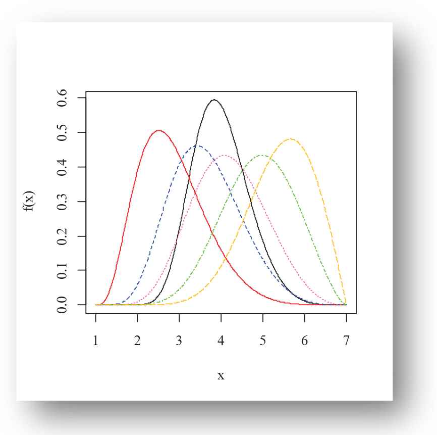
Density plot of exponentiated power function (EPF) distribution for Black(α = 5.1, β = 21.1), Red(α = 5.5, β = 4.2), Blue(α = 4.3, β = 7.3), Hotpink(α = 3.4, β = 8.4), Green(α = 2.5, β = 9.5), Goldenrod1(α = 2.0, β = 10.5) for m = 1, g = 7.
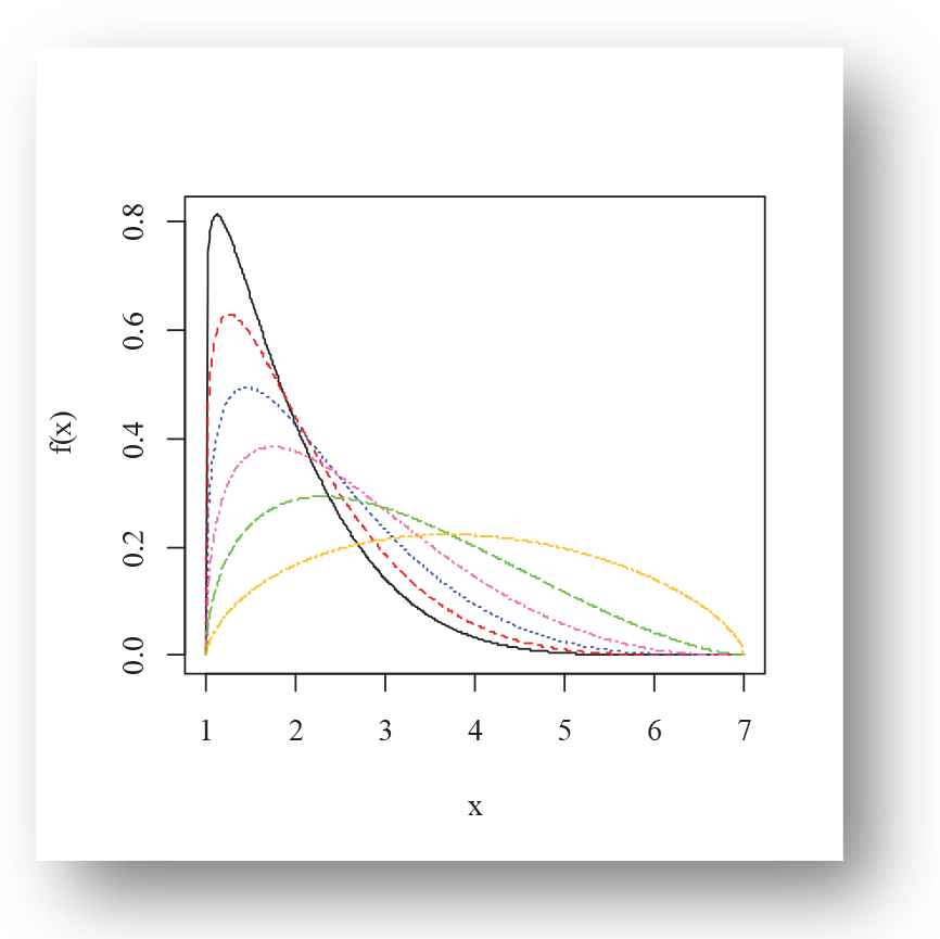
Density plot of exponentiated power function (EPF) distribution for Black(α = 6.1, β = 1.1), Red(α = 5.2, β = 1.2), Blue(α = 4.3, β = 1.3), Hotpink(α = 3.4, β = 1.4), Green(α = 2.5, β = 1.5), Goldenrod1(α = 1.6, β = 1.6) for m = 1, g = 7.
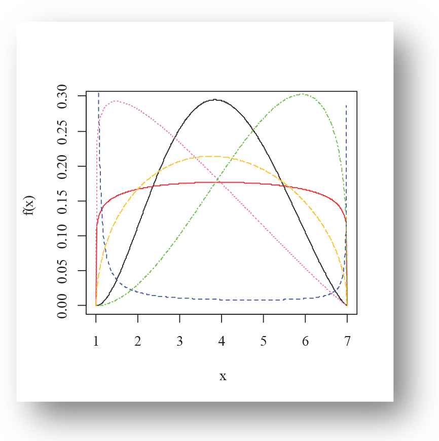
Density plot of exponentiated power function (EPF) distribution for Black(α = 2.3, β = 2.9), Red(α = 1.1, β = 1.1), Blue(α = 0.01, β = 0.02), Hotpink(α = 2.1, β = 1.1), Green(α = 1.3, β = 2.9), Goldenrod1(α = 1.5, β = 1.5) for m = 1, g = 7.
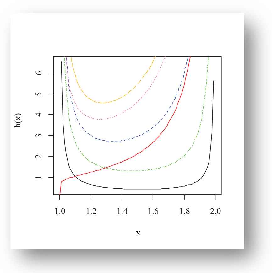
Failure rate function plot of exponentiated power function (EPF) distribution for Black(α = 0.009, β = 0.1), Red(α = 1.1, β = 1.1), Blue(α = 1.1, β = 0.1), Hotpink(α = 2.1, β = 0.3), Green(α = 0.2, β = 0.001), Goldenrod1(α = 2.5, β = 0.1) for m = 1, g = 7.
2.2. Linear Representations
Linear representation of PDF and CDF lead the calculations easier than the conventional integral calculation corresponding to determining the mathematical properties.
For power series expansion, if “β” is real noninteger and
Further properties of EPF distribution will be discussed by the conventional integral technique.
2.3. Limiting Behavior
Here we study the limiting behavior of distribution function, density function, reliability function and failure rate function of the EPF distribution present in Eqs. (1), (2), (3) and (4) at
Proposition 1.
Limiting behavior of distribution function, density function, reliability function and failure rate function of the EPF distribution at
Proposition 2.
Limiting behavior of distribution function, density function, reliability function and failure rate function of the EPF distribution at
Above limiting behaviors of distribution function, density function, reliability function and failure rate function illustrate the effect of parameters on the tail of the EPF distribution.
2.4. Moments and Its Associated Measures
Moments have a remarkable role in the discussion of distribution theory, to study the significant characteristics of a probability distribution.
Theorem 1.
Let
Proof from Eq. (2),
One can derive the mean of X by setting r = 1 in (7) and it is given by
For higher moments about the origin like 2nd, 3rd and 4th, it can be formulated by setting r = 2, 3 and 4 in the Eq. (7) respectively. Further to discuss the variability in X, the Fisher index
Corollary 1.
The relation between the ordinary moments and central moments is defined by
The s-th central moment of X is given by
The skewness and kurtosis of X are
Corollary 2.
The relation between ordinary moments and cumulants of a probability distribution is defined as
The r-th cumulants of X are given by
Furthermore, moment generating function can be written as
Moment generating function of X is given by
2.5. Quantile Function
Hyndman and Fan [16] introduced the concept of quantile function. The pth quantile function of
Quantile function of X is given by
One may obtain 1st quartile, median and 3rd quartile of X by setting p = 0.25, 0.5 and 0.75 in Eq. (8) respectively. Henceforth, to generate random numbers, we assume that CDF Eq. (1) follows uniform distribution u = U (0, 1).
2.6. Quantiles-Based Skewness, Kurtosis and Mean Deviation
Based on the quantile function, one can study the skewness (symmetry) and kurtosis (peakedness) of X by using the following useful measures introduced by Bowley [17] and Moors [18] respectively.
These descriptive measures are based on quartiles and octiles. Moreover, these measures are less reactive to the outliers and work more effectively for the distributions having the deficiency in moments.
Furthermore, quartile deviation of X is obtain by
In Figure 5, the Bowley skewness as a function of
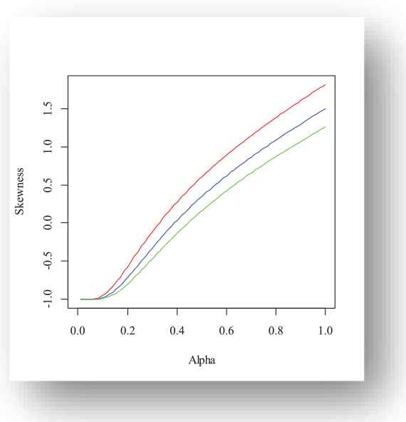
Red(β = 1.2), Blue(β = 1.9), Green(β = 3.5) for m = 1, g = 5.
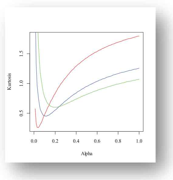
Red(β = 0.2), Blue(β = 0.3), Green(β = 0.4) for m = 1, g = 5.
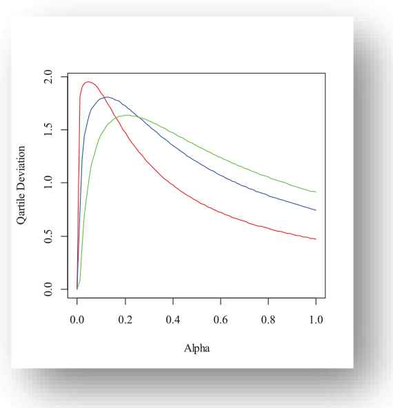
Red(β = 0.2), Blue(β = 0.3), Green(β = 0.4) for m = 1, g = 5.
2.7. Mode
Mode of EPF distribution is obtained by taking the first derivative of the PDF mention in Eq. (2)
2.8. Entropy
The disorderedness of a system is defined as entropy. The extended form of Shannon entropy is Rényi entropy as
Rényi entropy is described as
The simplified form of Rényi entropy when
The quadratic Rényi entropy is considered, as a special case of Rényi entropy. To obtain quadratic Rényi entropy of X, simply substitute
2.9. Order Statistics
In reliability analysis and life testing of a component in quality control, OS and its moments are considered as noteworthy measures. Let
By incorporating the Eqs. (1) and (2), i-th OS PDF of X is given by
The Eq. (9) is quite helpful in computing the w-th moment OS of the EPF distribution. Further, the minimum and maximum OS of
The w-th moment OS,
2.10. Stress–Strength Reliability
Let X1 and X2 be the strength and stress of a random component respectively. The life of the random component is described by the model known as the stress–strength reliability model. The inadequate and adequate working of a component depend on the conditions X2> X1 and X2< X1 respectively. It can be expressed as
Let
From Eqs. (1) and (2), reliability R is written as
3. PARAMETER ESTIMATION
In this section, we suggest the method of maximum likelihood estimation which provides the maximum information about the unknown model parameters.
From (2), the likelihood function,
To obtain the maximum likelihood estimates (MLEs) of the model parameters can be obtained by maximizing the above equation with respect to
The above two non-linear equations do not provide the analytical solution for MLEs and the optimum value of
3.1. Simulation Study
A simulation study can be executed by (a) Identity simulation; (b) Quasi-identity simulation; (c) Laboratory simulation; (d) Computer simulation. In this section, the performance of MLE's, we discuss by the following algorithm:
Step-1: A random sample x1, x2, x3,…, xn of sizes n = 25, 50, 100, 200 and 500 are generated from Eq. (8).
Step-2: Each sample is simulated 1000 times.
Step-3: The required results are obtained based on the different combinations of the parameters place in S-I(α = 0.5,
Step-4: Average MLEs and their corresponding standard errors (short S.Es) (present in parenthesis) are presented in Table 1.
| S-I |
S-II |
|||
|---|---|---|---|---|
| Parameters |
Parameters |
|||
| (Standard Errors) |
(Standard Errors) |
|||
| 25 | 0.4305 | 1.4049 | 3.0139 | 1.4049 |
| (0.1025) | (0.3881) | (0.7179) | (0.3882) | |
| 50 | 0.4914 | 1.5148 | 3.4395 | 1.5148 |
| (0.0821) | (0.3031) | (0.5747) | (0.3031) | |
| 100 | 0.5374 | 1.5624 | 3.7617 | 1.5624 |
| (0.0630) | (0.2221) | (0.4411) | (0.2222) | |
| 200 | 0.5206 | 1.4769 | 3.6441 | 1.4768 |
| (0.0440) | (0.1479) | (0.3080) | (0.1483) | |
| 500 | 0.4739 | 1.4460 | 3.3175 | 1.4460 |
| (0.0254) | (0.0908) | (0.1775) | (0.0908) | |
Average values of maximum likelihood estimates (MLEs) with standard errors (present in parenthesis) for various sample sizes.
Step-5: Biases and mean square errors (MSEs) are presented in Tables 2 and 3.
| S-III |
||||
|---|---|---|---|---|
| For |
For |
|||
| Bias | MSE | Bias | MSE | |
| 25 | 0.1909 | 0.4984 | 0.2196 | 0.3599 |
| 50 | 0.1034 | 0.1966 | 0.1128 | 0.1172 |
| 100 | 0.0259 | 0.0906 | 0.0506 | 0.0481 |
| 200 | 0.0155 | 0.0418 | 0.0394 | 0.0216 |
| 500 | −0.0068 | 0.0094 | 0.0179 | 0.0047 |
Bias and mean square errors (MSEs) for various sample sizes.
| S-IV |
||||
|---|---|---|---|---|
| For |
For |
|||
| Bias | MSE | Bias | MSE | |
| 25 | 0.4029 | 0.1429 | 0.4534 | 1.4515 |
| 50 | 0.0586 | 0.0571 | 0.2289 | 0.4349 |
| 100 | 0.0174 | 0.0265 | 0.1034 | 0.1736 |
| 200 | 0.0122 | 0.0123 | 0.0796 | 0.0781 |
| 500 | 0.0003 | 0.0027 | 0.0369 | 0.0166 |
Bias and mean square errors (MSEs) for various sample sizes.
Step-6: Mean, median, variance, skewness, kurtosis and confidence intervals (CIs) (90% and 95%) are presented in Tables 4–7.
| For |
S-III |
||||
|---|---|---|---|---|---|
| Mean | Median | Variance | Skewness | Kurtosis | |
| 25 | 2.6909 | 2.6040 | 0.4619 | 0.8309 | 4.0110 |
| 50 | 2.6034 | 2.5672 | 0.1859 | 0.1859 | 3.0492 |
| 100 | 2.5259 | 2.5022 | 0.0898 | 0.4047 | 3.0275 |
| 200 | 2.5155 | 2.5009 | 0.0416 | 0.4418 | 3.2494 |
| 500 | 2.4932 | 2.4912 | 0.0093 | 0.1690 | 3.1844 |
| For |
S-III |
||||
| Mean | Median | Variance | Skewness | Kurtosis | |
| 25 | 1.7196 | 1.5939 | 0.3117 | 1.7798 | 8.2574 |
| 50 | 1.6128 | 1.5735 | 0.1044 | 1.0428 | 4.9496 |
| 100 | 1.5506 | 1.5307 | 0.0456 | 0.6965 | 3.7277 |
| 200 | 1.5394 | 1.5268 | 0.0200 | 0.5001 | 3.1365 |
| 500 | 1.5179 | 1.5167 | 0.0041 | 0.1631 | 3.1463 |
Mean, median, variance, skewness and Kurtosis for various sample sizes.
| For |
S-IV |
||||
|---|---|---|---|---|---|
| Mean | Median | Variance | Skewness | Kurtosis | |
| 25 | 1.6029 | 1.5608 | 0.1323 | 0.7349 | 3.7258 |
| 50 | 1.5580 | 1.5388 | 0.0537 | 0.4042 | 2.9432 |
| 100 | 1.5174 | 1.5027 | 0.0262 | 0.3582 | 2.9546 |
| 200 | 1.5122 | 1.5023 | 0.0121 | 0.3922 | 3.1839 |
| 500 | 1.5002 | 1.4993 | 0.0027 | 0.1432 | 3.1876 |
| For |
S-IV |
||||
| Mean | Median | Variance | Skewness | Kurtosis | |
| 25 | 2.9533 | 2.6818 | 1.2460 | 1.9720 | 9.2736 |
| 50 | 2.7289 | 2.6453 | 0.3825 | 1.1625 | 5.4804 |
| 100 | 2.6034 | 2.5520 | 0.1629 | 0.7596 | 3.8927 |
| 200 | 2.5796 | 2.5516 | 0.0718 | 0.5571 | 3.2296 |
| 500 | 2.5369 | 2.5343 | 0.0152 | 0.1807 | 3.1734 |
Mean, median, variance, skewness and Kurtosis for various sample sizes.
| S-III |
||||
|---|---|---|---|---|
| Two-sided 90% CI |
Two-sided 95% CI |
|||
| For |
For |
For |
For |
|
| 25 | (2.6555, 2.7263) | (1.6904, 1.7486) | (2.6487, 2.7331) | (1.6850, 1.7542) |
| 50 | (2.5809, 2.6258) | (1.5960, 1.6296) | (2.5766, 2.6301) | (1.5927, 1.6329) |
| 100 | (2.5103, 2.5415) | (1.5394, 1.5616) | (2.5073, 2.5446) | (1.5373, 1.5638) |
| 200 | (2.5049, 2.5262) | (1.5320, 1.5468) | (2.5029, 2.5282) | (1.5307, 1.5482) |
| 500 | (2.4881, 2.4982) | (1.5144, 1.5213) | (2.4872, 2.4991) | (1.5138, 1.5220) |
Two-sided 90% and 95% confidence intervals (CIs) for α and
| S-IV |
||||
|---|---|---|---|---|
| Two-sided 90% CI |
Two-sided 95% CI |
|||
| n | For |
For |
For |
For |
| 25 | (1.5840, 1.6219) | (2.8952, 3.0114) | (1.5804, 1.6256) | (2.8841, 3.0226) |
| 50 | (1.5459, 1.5700) | (2.6967, 2.7611) | (1.5436, 1.5724) | (2.6905, 2.7672) |
| 100 | (1.5090, 1.5259) | (2.5824, 2.6244) | (1.5074, 1.5275) | (2.5784, 2.6284) |
| 200 | (1.5064, 1.5179) | (2.5656, 2.5935) | (1.5054, 1.5190) | (2.5629, 2.5962) |
| 500 | (1.4975, 1.5029) | (2.5305, 2.5433) | (1.4970, 1.5034) | (2.5292, 2.5446) |
Two-sided 90% and 95% confidence intervals (CIs) for α and
Step-7: Increase in the sample sizes reflects the consistent decrease in biases and MSEs, mean, median, variance, skewness, kurtosis and the two-sided 90% and 95% CI of the MLEs.
Step-8: Finally based on the results, we can declare that the method of maximum likelihood estimation works quite well for EPF.
4. APPLICATION
This section reports the application of EPF distribution. Accordingly, we consider two suitable lifetime datasets. The first dataset refers to the failure times of fifty devices put on life test at time zero discussed by Aarset [20] and the observations are 0.1, 0.2, 1.0, 1.0, 1.0, 1.0, 1.0, 2.0, 3.0, 6.0, 7.0, 11.0, 12.0, 18.0, 18.0, 18.0, 18.0, 18.0, 21.0, 32.0, 36.0, 40.0, 45.0, 45.0, 47.0, 50.0, 55.0, 60.0, 63.0, 63.0, 67.0, 67.0, 67.0, 67.0, 72.0, 75.0, 79.0, 82.0, 82.0, 83.0, 84.0, 84.0, 84.0, 85.0, 85.0, 85.0, 85.0, 85.0, 86.0, 86.0. The second dataset illustrates the thirty devices failure times discussed by Meeker and Escobar [21] and the observations are 275, 13, 147, 23, 181, 30, 65, 10, 300, 173, 106, 300, 300, 212, 300, 300, 300, 2, 261, 293, 88, 247, 28, 143, 300, 23, 300, 80, 245, 266. The EPF distribution compares to its competing models based on the criteria: -log-likelihood (-LogL), Akaike information criterion (AIC), Bayesian information criterion (BIC), consistent Akaike information criterion (CAIC), Hannan-Quinn information criterion (HQIC). The following goodness-of-fit statistics comprising Anderson-Darling (A*) and Cramer-von Mises (W*) are used to study the fit of EPF distribution to the data. The minimum value of (-LogL), AIC, BIC, CAIC, HQIC, A* or W* can be helpful to declare the model as best fit to the data.
Numerous facts and figures of proposed and competing models are presented in Tables 8–12, corresponding to the Aarset [20] and Meeker and Escobar [21] datasets. Table 8 illustrates the various descriptive statistics. Tables 9 and 11 describe the parameters estimates and their standard errors (present in parenthesis). Furthermore, Tables 10 and 12 express the various selection criterions and goodness-of-fit statistics. The EPF distribution satisfies the criteria of a better fit model based on the results. Consequently, we declare the EPF distribution is a better fit in its competing models on both the datasets.
| Data | Min. | 1st Quartile | Median | Mean | 3rd Quartile | Maximum |
|---|---|---|---|---|---|---|
| Aarset | 0.10 | 13.50 | 48.50 | 45.67 | 81.25 | 86.00 |
| Meeker and Escobar | 2.00 | 68.75 | 196.50 | 177.03 | 298.25 | 300.00 |
Descriptive information.
| Models | Estimates (Standard Errors) |
|||||
|---|---|---|---|---|---|---|
| EPF | 0.33 | 0.45 | − | − | − | − |
| (0.0781) | (0.0742) | |||||
| KPF | 0.37 | 0.41 | − | − | 1.05 | − |
| (23.4742) | (0.0678) | (67.1407) | ||||
| OGEP | 3.33 | 0.14 | − | − | − | 0.05 |
| (0.6629) | (0.0283) | (0.0174) | ||||
| WPF | − | 1.49 | 0.73 | − | 1.05 | − |
| (0.4886) | (1.2097) | (67.1407) | ||||
| MOPF | 7.62 | 0.26 | − | − | − | − |
| (5.7076) | (0.1544) | |||||
| GPF | 0.58 | − | − | − | − | − |
| (0.0817) | ||||||
EPF = exponentiated power function; GPF = generalized power function; WPF = Weibull power function; KPF = Kumaraswamy power function; MOPF = Marshall-Olkin power function, OGEPF = odd generalized exponentiated power function.
Parameter estimates and standard errors in parenthesis for Aarset dataset for
| Model | -LogL | AIC | BIC | HQIC | CAIC | W* | A* |
|---|---|---|---|---|---|---|---|
| EPF | 199.17 | 402.34 | 406.16 | 403.79 | 402.59 | 0.0434 | 0.3579 |
| KPF | 201.58 | 409.16 | 414.89 | 411.34 | 409.68 | 0.0442 | 0.3750 |
| OGEP | 204.12 | 414.24 | 419.97 | 416.42 | 414.76 | 0.0374 | 0.3102 |
| WPF | 205.18 | 416.35 | 422.09 | 418.54 | 416.87 | 0.0459 | 0.3799 |
| MOPF | 212.55 | 429.11 | 432.93 | 430.56 | 429.36 | 0.1179 | 0.8264 |
| GPF | 213.56 | 429.12 | 431.03 | 429.85 | 429.20 | 0.0482 | 0.3628 |
EPF = exponentiated power function; GPF = generalized power function; WPF = Weibull power function; KPF = Kumaraswamy power function; MOPF = Marshall-Olkin power function, OGEPF = odd generalized exponentiated power function.
Information criterions and goodness-of-fit statistics for Aarset dataset.
| Model | Estimates (Standard Errors) |
|||||
|---|---|---|---|---|---|---|
| EPF | 0.15 | 0.41 | − | − | − | |
| (0.0464) | (0.0849) | |||||
| KPF | 0.50 | 0.22 | − | − | 0.67 | − |
| (62.6313) | (0.0446) | (83.6549) | ||||
| OGEP | 1.44 | 0.21 | − | − | − | 0.005 |
| (0.58) | (0.05) | (0.003) | ||||
| WPF | − | 3.38 | 0.81 | 0.21 | − | − |
| (1.3170) | (0.2509) | (0.0487) | ||||
| MOPF | 11.80 | 0.28 | − | − | − | − |
| (13.33) | (0.27) | |||||
| GPF | 0.23 | − | − | − | − | − |
| (0.0507) | ||||||
EPF = exponentiated power function; GPF = generalized power function; WPF = Weibull power function; KPF = Kumaraswamy power function; MOPF = Marshall-Olkin power function, OGEPF = odd generalized exponentiated power function.
Parameter estimates and standard errors in parenthesis for Meeker and Escobar dataset for
| Model | -LogL | AIC | BIC | HQIC | CAIC | W* | A* |
|---|---|---|---|---|---|---|---|
| EPF | 119.63 | 243.26 | 246.06 | 244.15 | 243.70 | 0.09 | 0.85 |
| KPF | 125.21 | 256.41 | 260.62 | 257.76 | 257.34 | 0.19 | 1.45 |
| WPF | 152.58 | 311.15 | 315.36 | 312.50 | 312.08 | 0.08 | 0.75 |
| OGEP | 154.37 | 314.74 | 318.94 | 316.08 | 315.66 | 0.28 | 1.92 |
| GPF | 154.37 | 314.74 | 318.94 | 316.08 | 315.66 | 0.28 | 1.92 |
| MOPF | 165.53 | 335.06 | 337.87 | 335.96 | 335.51 | 0.34 | 2.30 |
EPF = exponentiated power function; GPF = generalized power function; WPF = Weibull power function; KPF = Kumaraswamy power function; MOPF = Marshall-Olkin power function, OGEPF = odd generalized exponentiated power function.
Information criterions and goodness-of-fit statistics for Meeker and Escobar dataset.
Competing Models
| Abbr. | Model | Parameters/Variable Range | Reference |
|---|---|---|---|
| GPF | Saran and Pandey [3] | ||
| WPF | Tahir et al. [9] | ||
| KPF | Abdul-Moniem [13] | ||
| MOPF | Okorie et al. [12] | ||
| OGEPF | Tahir et al. [22] |
GPF = generalized power function; WPF = Weibull power function; KPF = Kumaraswamy power function; MOPF = Marshall-Olkin power function, OGEPF = odd generalized exponentiated power function.
The following fitted PDFs, CDFs, competing models, Kaplan Meier survival and probability probability (PP) plots are drafted over empirical histogram for Aarset data, presented in Figures 8–11, respectively.
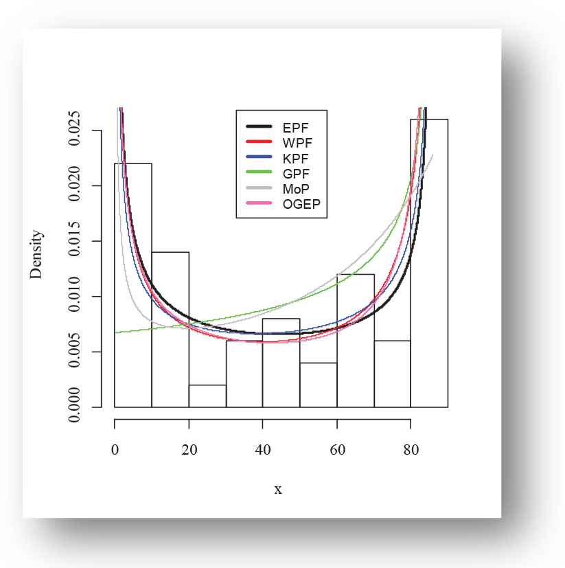
Empirical fitted density finction plot of exponentiated power function (EPF) distribution for Aarset data
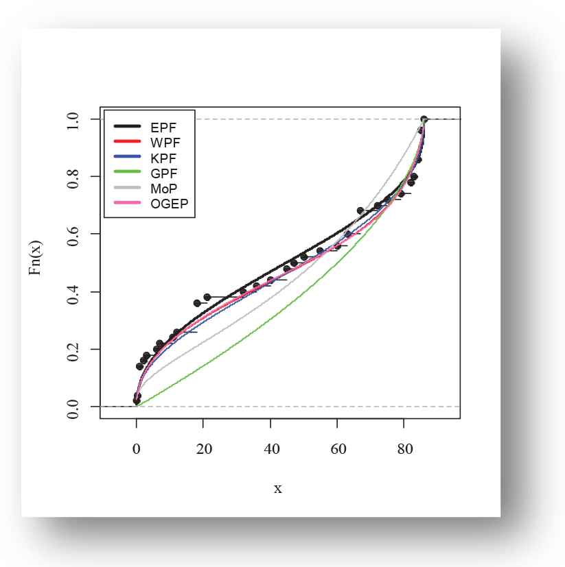
Empirical fitted distribution function plot of exponentiated power function (EPF) distribution for Aarset data
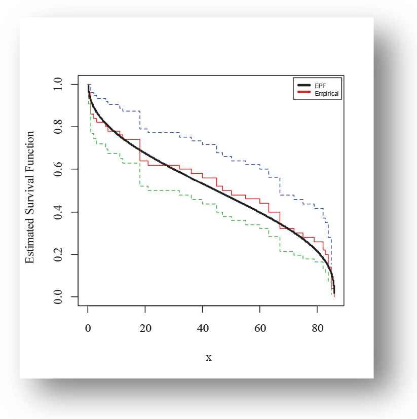
Kaplan-Meier survival finction plot of exponentiated power function (EPF) distribution for Aarset data
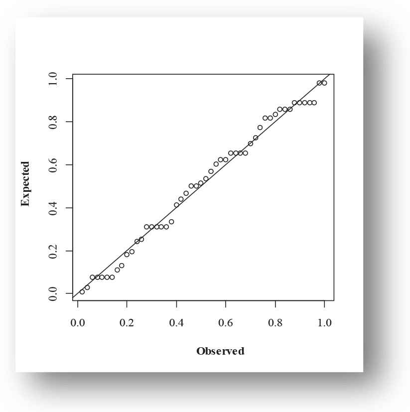
Probability-probability (PP) plot of exponentiated power function (EPF) distribution for Aarset data
The following fitted PDFs, CDFs, competing models, Kaplan Meier survival and PP plots are drafted over empirical histogram for Meeker and Escobar data, presented in Figures 12–15, respectively.
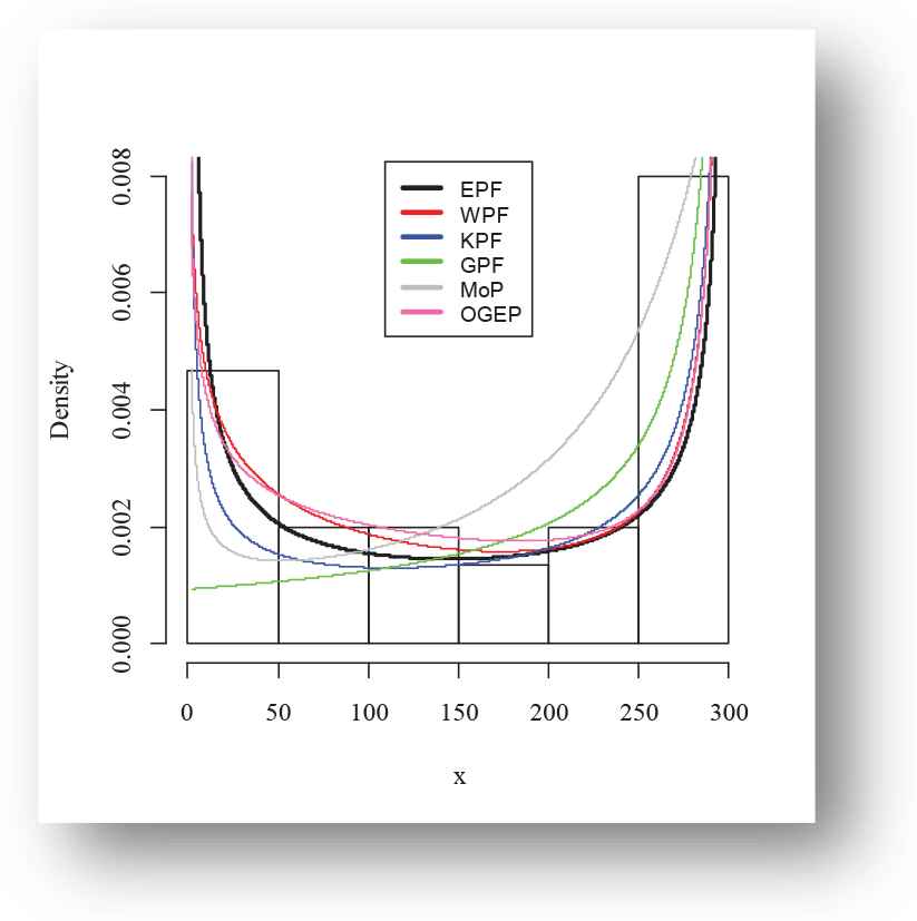
Empirical fitted density finction plot of exponentiated power function (EPF) distribution for Meeker and Escobar data
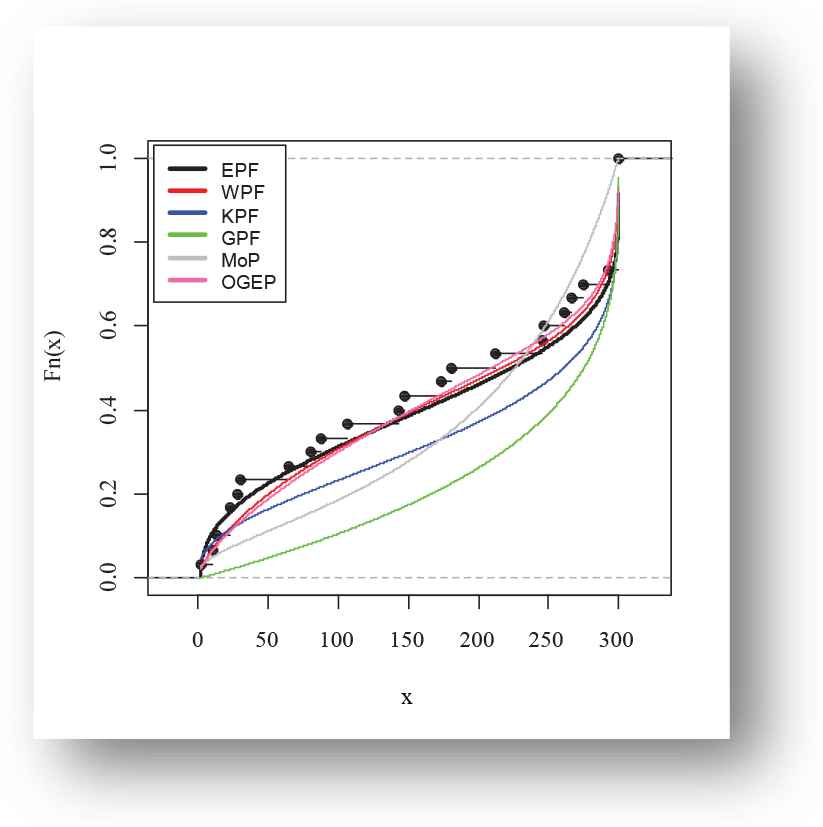
Empirical fitted distribution function plot of exponentiated power function (EPF) distribution for Meeker and Escobar data
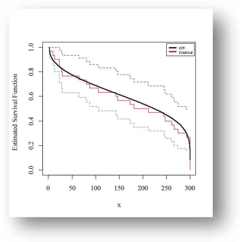
Kaplan-Meier survival finction plot of exponentiated power function (EPF) distribution for Meeker and Escobar data
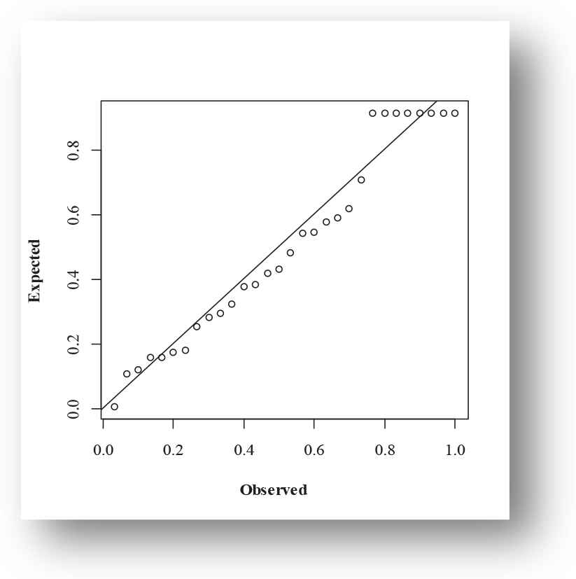
Probability-Probability (PP) plot of exponentiated power function (EPF) distribution for Meeker and Escobar data
5. CONCLUSION
In this article, we have developed a flexible model that demonstrates the bathtub-shaped density and failure rate functions and addresses the most efficient and consistent results, over the data follows to the bathtub-shaped phenomena. The proposed distribution is the exponentiated form of generalized power function distribution and it is referred to as the exponentiated power function (EPF) distribution. Numerous structural and reliability measures are derived and discussed. Model parameters are estimated by the method of maximum likelihood estimation and the Monte Carole simulation is carried out as well to investigate the performance of the MLEs. Two datasets from engineering sectors discussed by Aarset and Meeker and Escobar, are used to reveal the superiority of EPF distribution over its competing models.
CONFLICT OF INTEREST
There are no conflicts of interest for any of the authors.
AUTHORS' CONTRIBUTIONS
All authors had access to the data and a role in writing the manuscript.
ACKNOWLEDGMENTS
The authors are grateful to the editor and anonymous reviewers for their constructive comments and valuable suggestions which certainly improved quality of the paper.
REFERENCES
Cite this article
TY  - JOUR
AU  - Muhammad Zeshan Arshad
AU  - Muhammad Zafar Iqbal
AU  - Munir Ahmad
PY  - 2020
DA  - 2020/07/03
TI  - Exponentiated Power Function Distribution: Properties and Applications
JO  - Journal of Statistical Theory and Applications
SP  - 297
EP  - 313
VL  - 19
IS  - 2
SN  - 2214-1766
UR  - https://doi.org/10.2991/jsta.d.200514.001
DO  - 10.2991/jsta.d.200514.001
ID  - Arshad2020
ER  -