Journal of Statistical Theory and Applications

Volume 19, Issue 3, September 2020, Pages 342 - 351

EBC-Estimator of Multidimensional Bayesian Threshold in Case of Two Classes

Authors
Oksana Kubaychuk*, ORCID
Institute of Physics and Technology, National Technical University of Ukraine «Igor Sikorsky Kyiv Polytechnic Institute», 37, Prosp. Peremohy, Kyiv, 03056, Ukraine
Corresponding Author
Oksana Kubaychuk
Received 24 April 2020, Accepted 27 July 2020, Available Online 8 September 2020.
DOI
10.2991/jsta.d.200824.001How to use a DOI?
Keywords
Estimator; Multidimensional Bayesian threshold; Mixture with varying concentrations
Abstract

Some threshold-based classification rules in case of two classes are defined. In assumption, that a learning sample is obtained from a mixture with varying concentration, the empirical-Bayesian classification (EBC)-estimator of multidimensional Bayesian threshold is constructed. The conditions of convergence in probability of estimator are found.

Copyright
© 2020 The Authors. Published by Atlantis Press B.V.
Open Access
This is an open access article distributed under the CC BY-NC 4.0 license (http://creativecommons.org/licenses/by-nc/4.0/).

1. INTRODUCTION

The model of a mixture of several probability distributions was mentioned for the first time by Newcomb [1] and Pearson [2]. Such mixtures naturally arise in many areas. In particular, in the theory of reliability and time of life, mixtures of gamma distributions [3] are used. Examples of the use of mixtures of normal distributions in the processing of biological and physiological data are given in [4]. In Slud [5], a mixture of two exponential distributions is used to describe the debugging process of the software. Some applications of the model of mixtures in medical diagnostics were given in [6,7].

The technique of a nonparametric analysis of mixtures where concentrations changes from observation to observation develops, actively. The problem of distributions estimating in case at known concentrations is considered in the works of Maiboroda [8,9]. Estimates of concentrations in two-component mixtures in work [10]. Works by Sugakova [11] and Ivanko [12] are devoted to the evaluation of component distribution densities. The correction algorithms for weighted empirical distribution functions are proposed in [13].

For the theoretical study of problems of nonparametric regression the nonhomogeneous weighted empirical distribution functions used by Stoune [14]. These were applied by Maiboroda in the tasks of analyzing the mixture. In particular, in Maiboroda [8] found conditions under which the weighted empirical distribution functions are unbiased and minimal estimators of unknown distribution functions of components of the mixture.

Object classification by its numerical characteristic is an important theoretical problem and has practical significance, for example, the definition of a person as “not healthy,” if the temperature of its body exceeds 37°C. To solve this problem we consider the threshold-based rule of type

gt(ξ)=1,ξt,2,ξ>t.

According to this rule, an object is classified to the first class if its characteristic does not exceed a threshold t= 37°C; otherwise, an object is classified to belong to the second class. The empirical-Bayesian classification (EBC) [15,16] and minimization of the empirical risk (MER) [17,18] are widely used methods to estimate the best threshold. The case when the learning sample is obtained from a mixture with varying concentrations is considered in [19] and the asymptotic of both methods of estimating is investigated.

However, it is often necessary to classify an object in case of more than one threshold, for example, the definition of a person as “not healthy,” if the temperature of its body exceeds 37°C or lower than 36°C. Another example: the person is sick, if the level of its hemoglobin exceeds 84 units or lower than 72 units. Accordingly, one can apply the classifiers of type

gt1,t21(ξ)=1,ξt1,t2,2,ξt1,t2
or
gt1,t22(ξ)=1,ξt1,t2,2,ξt1,t2.

In particular, this problem is discussed in [20,21].

The case of two thresholds and three prescribed classes deserves special attention. An example is the classification of the disease stages. Thus, during the diagnosis of breast cancer a tumor marker CA 15-3 is used. If the value is less than 22 IU/mL, then the person is healthy; if its level is in the range from 22 to 30 IU/mL—precancerous conditions can be diagnosed; if the index is above 30 IU/mL—patient has cancer. When solving some technical problems it is needed to consider the substance in its various aggregate forms: gaseous, liquid, solid. The transition from state to state occurs at a specific temperature. According to this, a boiling point and a melting point are used. Accordingly, 6 classifiers of forms

gt1,t2(ξ)=1,ξ<t1,2,t1ξt2,3,ξ>t2
can be applied. This partial case was studied in [22].

2. SETTING OF THE PROBLEM

The problem of classification of an object O from the observation of its numerical characteristic ξ=ξ(O) is studied. We assume that the object may belong to one of two prescribed classes. An unknown class number containing O is denoted by ind(O). A classification rule (briefly, classifier) is a function g:n{1,2} that assigns a value to ind(O) by using characteristic ξ. In general, classification rule is defined as a general measurable function, but we restrict the consideration in this paper to the so-called threshold-based classification rules of the forms

g2m1,t1(ξ)=1,ξk=1m1,m>1t2k,t2k+1(,t1],2,ξk=1m1,m>1t2k1,t2kt2m1,+,
g2m1,t2(ξ)=1,ξk=1m1,m>1t2k1,t2kt2m1,+,2,ξk=1m1,m>1t2k,t2k+1,t1,
if n=2m1,  m and
g2m,t1(ξ)=1,ξk=1m1,m>1t2k,t2k+1,t1t2m,+,2,ξk=1mt2k1,t2k,
g2m,t2(ξ)=1,ξk=1mt2k1,t2k,2,ξk=1m1,m>1t2k,t2k+1,t1t2m,+,
if n=2m,  m, where t=t1,t2,tn is the multidimensional threshold.

The a priori probabilities pi=P(ind(O)=i), i=1,2 are assumed to be known. The characteristic ξ is assumed to be random, and its distribution depends on ind(O):P(ξ(O)<x|ind(O)=i)=Hi(x), i=1,2. The distributions Hi are unknown, but they have continuous densities hi with respect to the Lebesgue measure.

The family of classifiers is denoted by G=gt:tn.

Let, n=2m1,  m then the probability of error of such a classification rules are given by

Lg2m1,t1=L2m11(t)=Pgt1(ξ(O))ind(O)=i=12Pind(O)=iPgt1(ξ(O))=3i|ind(O)=i=p1k=1mH1t2kH1t2k1+p11H1t2m+1+p2k=1mH2t2k+1H2t2k+p2H2t1
Lg2m1,t2=L2m12(t)=Pgt2(ξ(O))ind(O)=i=12Pind(O)=iPgt2(ξ(O))=3i|ind(O)=i=p1k=1mH1t2k+1H1t2k+p1H1t1+p2k=1mH2t2kH2t2k1+p21H2t2m+1.

Analogically, for n=2m,  m:

Lg2m,t1=L2m1(t)=Pg2m,t1(ξ(O))ind(O)=i=12Pind(O)=iPg2m,t1(ξ(O))=3i|ind(O)=i=p1k=1mH1t2kH1t2k1+p21H2t2m+p2k=1m1,m>1H2t2k+1H2t2k+p2H2t1
Lg2m,t2=L2m2(t)=Pg2m,t2(ξ(O))ind(O)=i=12Pind(O)=iPg2m,t2(ξ(O))=3i|ind(O)=i=p2k=1mH2t2kH2t2k1+p1H1t1+p1k=1mH1t2k+1H1t2k+p11H1t2m

A classification rule gBG is called a Bayesian classification rule in the class G, if L(g) attains its minimum at gBgB=argmingGL(gt). The threshold tB for a Bayesian classification rule is called the Bayesian threshold:

tB=argmintnL(t)(1)

Let,

ti=argmintLi,2m11(t),   t1<t2<<t2m1

Denote Bayesian threshold for classifier g2m1,t1:

t2m11B=argmint2m1L2m11(t)=t1,t2,,t2m1,
where
Li,2m11(t)=(1)ip1H1(t)p2H2(t),   i=1,,2m2,   m, and
L2m1,2m11(t)=p1p1H1(t)p2H2(t).

Analogically, let

ti=argmintLi,2m12(t),   t1<t2<<t2m1

For g2m1,t2:

t2m12B=argmint2m1L2m12(t)=t1,t2,,t2m1,
where
Li,2m12(t)=(1)ip1H1(t)+p2H2(t),   i=1,,2m2,   m, and
L2m1,2m12(t)=p2+p1H1(t)p2H2(t).

Let,

ti=argmintLi,2m1(t),   t1<t2<<t2m

For g2m,t1:

t2m1B=argmint2mL2m1(t)=t1,t2,,t2m,
where
Li,2m1(t)=(1)ip1H1(t)p2H2(t),   i=1,,2m1,   m, and
L2m,2m1t2=p2+p1H1(t2m)p2H2(t2m)

Let,

ti=argmintLi,2m2(t),   t1<t2<<t2m

For g2m,t2:

t2m2B=argmint2mL2m2(t)=t1,t2,,t2m,
where
Li,2m2(t)=(1)ip1H1(t)+p2H2(t),   i=1,,2m1,   m
L2m,2m2(t)=p1p1H1(t)p2H2(t).

Denote

Ln1(t)=L1,n1t1+L2,n1t2++Ln,n1tn,
Ln2(t)=L1,n2t1+L2,n2t2++Ln,n2tn,
where n=2m1,  m or n=2m,  m.

When determining the best threshold, one faces the problem of estimating the threshold by using a learning sample, whose members are classified correctly. We consider the Bayesian empirical classification method, in assumption, that a learning sample is obtained from a mixture with varying concentration.

The distribution functions Hs (and, of course, densities hs) are assumed to be unknown. One can estimate these functions from the data ΞN=ξj:Nj=1N being a sample from a mixture with varying concentration, where ξj:N are independent if N is fixed and

Pξj:N<x=wj:NH1(x)+1wj:NH2(x).

Here wj:N is a known concentration in the mixture of objects of the first class at the moment when an observation j is made [23].

To estimate the distribution functions Hs, we use weighted empirical distribution functions

HsN(x)=1Nj=1Naj:Ns1ξj<x(2)
where 1A is the indicator an event A and aj:Ns are known weight coefficients:
aj:N1=1ΔN1SN1wj:N+SN2SN1,   aj:N2=1ΔNSN2SN1wj:N,
SNk=1Nj=1Nwj:Nk,   k=1,2,   ΔN=SN2SN12
(see [23]).

One can apply kernel estimators to estimate the densities of distributions:

hsN(x)=1NkNj=1Naj:NsKxξj:NkN,
where K is a kernel (the density of some probability distribution) and kN is a smoothing parameter [11,24].

The empirical-Bayesian estimator is constructed as follows. At first, one determines the set TN of all solutions of the equation

p1h1N(t)p2h2N(t)=0,   t1<t2<<tn,(3)
where n=2m1,  m or n=2m,  m for every N.

Second, one chooses

tN,n1EBC=argmintTNLN,1,n1(t),argmintTNLN,2,n1(t),,argmintTNLN,n,n1(t)
as an estimator for tB, where
LN,i,2m11(t)=(1)ip1H1N(t)p2H2N(t),   i=1,,2m2,   m,
LN,2m1,2m11(t)=p1p1H1N(t)p2H2N(t);
LN,i,2m1(t)=(1)ip1H1N(t)p2H2N(t),   i=1,,2m1,   m,
LN,2m,2m1(t)=p2+p1H1N(t)p2H2N(t),
tN,i,n1EBC=argmintTNLN,i,n1(t),   i=1,,n,   n=2m(n=2m1),
therefore
tN,n1EBC=tN,1,n1EBC,tN,2,n1EBC,,tN,n,n1EBC;
LN,n1(t)=LN,1,n1t1+LN,2,n1t2++LN,n,n1tn,
where n=2m1,  m or n=2m,  m, or
tN,n2EBC=argmintTNLN,1,n2(t),argmintTNLN,2,n2(t),,argmintTNLN,n,n2(t),
where
LN,i,2m12(t)=(1)ip1H1N(t)+p2H2N(t),   i=1,,2m2,   m,
LN,2m1,2m12(t)=p2+p1H1N(t)p2H2N(t);
LN,i,2m2(t)=(1)ip1H1N(t)+p2H2N(t),   i=1,,2m1,   m,
LN,2m,2m2(t)=p1p1H1N(t)p2H2N(t),
tN,i,n1EBC=argmintTNLN,i,n1(t),   i=1,,n,  n=2m(n=2m1),
and
tN,n1EBC=tN,1,n1EBC,tN,2,n1EBC,,tN,n,n1EBC.
LN,n2(t)=LN,1,n2t1+LN,2,n2t2++LN,n,n2tn,
where n=2m1,  m or n=2m,  m.

An example of multidimensional threshold in case of two classes is shown on Figures 1 and 2 (Mathcad v.13 was used).

Figure 1

Three-dimensional threshold: h1 = 0.5N(0,1) + 0.5N(4,1), h2 = 0.4N(2,1) + 0.6N(6,1), p1 = 0.3, p2 = 0.7.

Figure 2

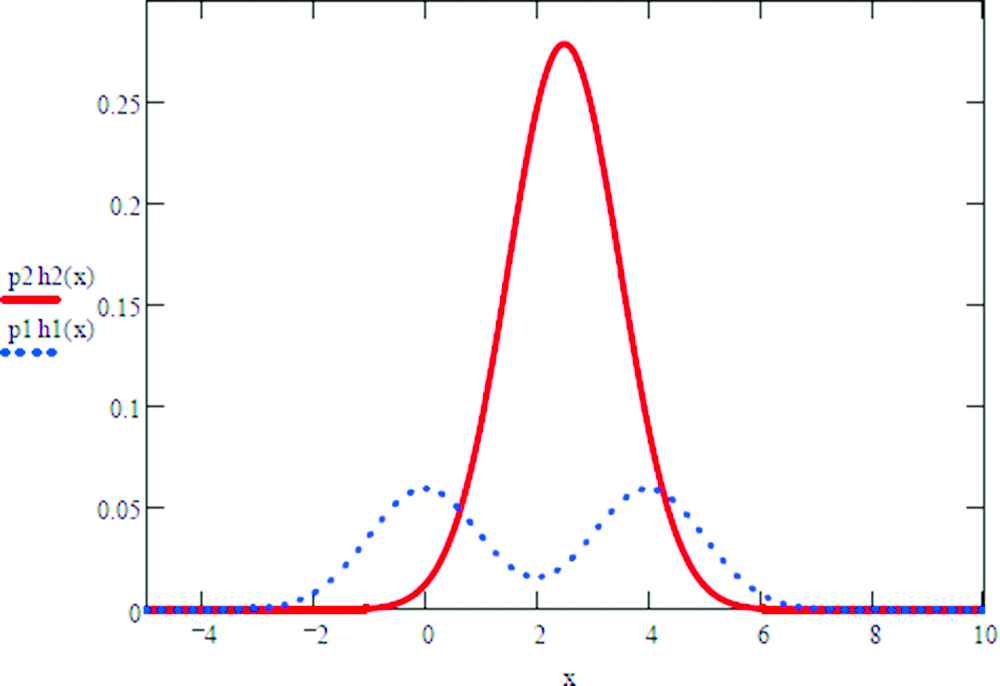
Two-dimensional threshold: h1 = 0.5N(0,1) + 0.5N(4,1), h2 = N(2.5,1), p1 = 0.3, p2 = 0.7.

3. MAIN RESULTS

3.1. Choice of Classifier

The choice of the classifier g2m1,t1g2m,t1 or g2m1,t2g2m,t2 depends on the smallest root of the equation

p1h1p2h2=0.(4)

Theorem 3.1.1.

If root of (4) minimizes L1,2m11L1,2m1, then the classifier g2m1,t1g2m,t1 is selected, but if it minimizes L1,2m12L1,2m2, then it is selected g2m1,t2g2m,t2.

Proof.

The statement follows from the properties Li,2m11=Li,2m12,i=1,,2m2 and Li,2m1=Li,2m2,i=1,,2m1.

Remark 3.1.1.

L2m1,2m11=L2m1,2m12+p1+p2 and L2m,2m1=L2m,2m2+p1+p2.

The next theorem can be proved analogically to Theorem 3.1.1.

Theorem 3.1.2.

If root of (3) minimizes LN,1,2m11LN,1,2m1, then the tN,n1EBC is selected, but if it minimizes LN,1,2m12LN,1,2m2, then it is selected tN,n2EBC.

Proof.

The statement follows from the properties LN,i,2m11=LN,i,2m12,i=1,,2m2 and LN,i,2m1=LN,i,2m2,i=1,,2m1.

Remark 3.1.2.

LN,2m1,2m11=LN,2m1,2m12+p1+p2 and LN,2m,2m1=LN,2m,2m2+p1+p2.

Remark 3.1.3.

As follows from [2528], we can use the improved weighted distribution function if some coefficients are negative in (2).

3.2. The Convergence in Probability of EBC-Estimator

In what follows we assume that

(A). The threshold tBn,n=2m1(n=2m),m exists, is a unique of the global minimum of Ln1(t),n=2m1(n=2m),m or Ln2(t),n=2m1(n=2m),m (ti,nB is a global minimum point of Li,n1ti,i=1,,n,n=2m1(n=2m),m or Li,n2ti,i=1,,n,n=2m1(n=2m),m).

(Bk). The limits Sl=limnSNl, l=1,2,k, exists and Δ=S2Sl2>0.

Lemma 3.2.1.

Let conditions (A) and (Bk) hold. Assume that densities h1 and h2 exist and are continuous, kN0, NkN, K is a continuous function, and

d2:=K2(t)dt<.

Then PANδi1,N, for δi>0, where ANδi=ti:|titi,nB|δi,uNti=0 and uN(x):=p2h2N(x)p1h1N(x), i=1,,n.

Proof.

According to Theorem 1 of [11], the assumptions of the theorem imply that hsNxhsx,s=1,2 in probability at every point x. Therefore,

uN(x):=p2h2N(x)p1h1N(x)u(x):=p2h2(x)p1h1(x)
in probability. For δ>0, let
ANδi=ti:|titi,nB|δi,uNti=0.

Now we shall that

PANδi1,N.(5)

Since, ti,nB is a point of minimum of Li,n1tor Li,n2t, i=1,,n,n=2m1(n=2m),m, and Li,n1(t)=u(t) or Li,n1(t)=u(t) (similarly, Li,n2(t)), depending on the parity or the oddness of i, is a continuous function, u(t) changes its sign in a neighborhood of the point ti,nB. This means that there are ti and ti+ such that

ti,nBδi<ti<ti,nB<ti+<ti,nB+δi,i=1,,n,n=2m1(n=2m),m
and utiuti+<0.

Thus, PuNtiuNti+<01. Since uN is a continuous function, uNtiuNti+<0ANδi. Therefore (5) is proved.

Lemma 3.2.2.

Let assumptions of Lemma 3.2.1 for δi>0,0<δi<δi hold. Then

PBi,N1 as N,
where
Bi,N=inftti,nBδi,  ti,nB+δiLN,i,n1t>Li,n1ti,nB+ε2>suptti,nBδi,  ti,nB+δiLN,i,n1t,i=1,,n,n
for g2m1,t1org2m,t1 and
Bi,N=inftti,nBδi,  ti,nB+δiLN,i,n2t>Li,n2ti,nB+ε2>suptti,nBδi,  ti,nB+δiLN,i,n2t,i=1,,n,n
for g2m1,t2org2m,t2.

Proof.

Fix δi, i=1,,n,n. Since Li,n1 (Li,n2) are continuous functions on , i=1,,n,n,

Li,2m11=0,i=1,,2m2Li,2m12=0,i=1,,2m2,
Li,2m1=0,i=1,,2m1Li,2m2=0,i=1,,2m1,
Li,2m11+=(1)ip1p2,i=1,,2m2Li,2m12+=(1)ip1+p2,i=1,,2m2,
Li,2m1+=(1)ip1p2,i=1,,2m1Li,2m2+=(1)ip1+p2,i=1,,2m1,
L2m1,2m11=p1,L2m1,2m11+=p2,L2m,2m1=p2,L2m,2m1+=p1,
L2m1,2m12=p2,L2m1,2m12+=p1,L2m,2m2=p1,L2m,2m2+=p2
and condition (A) holds. Moreover δi>0εi such that Li,n1ti>Li,n1ti,nB+εi,  i=1,,n (or Li,n2ti>Li,n2ti,nB+εi,  i=1,,n) for all ti for which |titi,nB|>δi.

Choose 0<δi<δi so that

Li,n1ti<Li,n1ti,nB+εi4or Li,n2ti<Li,n2ti,nB+εi4,i=1,,n,n
for all titi,nBδi,ti,nB+δi. Denote
Bi,N=inftti,nBδi,ti,nB+δiLN,i,n1t>Li,n1ti,nB+ε2>suptti,nBδi,ti,nB+δiLN,i,n1t,i=1,,n,n
for g2m1,t1g2m,t1 and
Bi,N=inftti,nBδi,  ti,nB+δiLN,i,n2t>Li,n2ti,nB+ε2>suptti,nBδi,  ti,nB+δiLN,i,n2t,i=1,,n,n
for g2m1,t2g2m,t2.

Fix an arbitrary λi>0. Using the uniform convergence of LN,i,n1 to Li,n1 (or LN,i,n2 to Li,n2), we obtain the necessary statement for sufficiently large N for according Bi,N, pBi,N>1Ai/2.

Theorem 3.2.1.

Assume that conditions of Lemma 3.2.1 hold. Then tN,n1EBCtB (or tN,n2EBCtB) in probability as N, namely tN,i,n1EBCtiB, i=1,,n,n (or tN,i,n2EBCtiB, i=1,,n,n) in probability as N.

Proof.

Since (5) PANδi>1λi2 for sufficiently large N. If the event ANδi occurs, then there exists

tiTNti,nBδi,ti,nB+δi
such that LN,i,n1ti<LN,i,n1ti for all titi,nBδi,  ti,nB+δi given the event Bi,N occurs (or LN,i,n2ti<LN,i,n2ti for all titi,nBδi,  ti,nB+δi). Therefore,
PtN,i,n1EBCti,nB<δPANδiBi,N1λi2+1λi21=1λi
and
PtN,i,n2EBCti,nB<δPANδiBi,N1λi2+1λi21=1λi
given the event Bi,N occurs for sufficiently large N, i=1,,n,n, taking into account that
PANδiBi,N=PANδi+PBi,NPANδiBi,NPANδi+PBi,N1.

This completes the proof of the theorem, since λi, i=1,,n,n are arbitrary.

4. CONCLUSION

In this paper, we found the conditions of convergence in probability of the estimator for the Bayesian threshold constructed by the method of empirical-Bayesian classification for a sample from a mixture with variable concentrations.

CONFLICT OF INTEREST

The author has no conflicts of interest to declare.

ACKNOWLEDGMENTS

I thank the reviewers whose insightful comments helped me to improve this paper.

REFERENCES

9.R.E. Maiboroda, Theory Probab. Math. Stat., Vol. 59, 1999, pp. 121-128.
10.R.E. Maıboroda, Theory Probab. Math. Stat., Vol. 46, 1993, pp. 71-75.
11.O.V. Sugakova, Theory Probab. Math. Stat., Vol. 59, 1999, pp. 161-171.
12.Yu.O. Ivan'ko, Visn. Mat. Mekh. Kyïv. Univ. Im. Tarasa Shevchenka, Vol. 9, 2003, pp. 29-35.
15.L. Devroye and L. Gyorfi, Nonparametric Density Estimation, The L1 View, John Wiley & Sons, Inc., New York, NY, USA, 1985.
17.V.N. Vapnik, Yu.I. Zhuravlev (editor), Pattern Recognition, Classification, Prediction, Nauka, Moscow, Russia, Vol. 1, 1989, pp. 17-81.
20.O. Kubajchuk, Visn. Mat. Mekh. Kyiv. Univ. Im. Tarasa Shevchenka, Vol. 19, 2008, pp. 47-51.
21.O.O. Kubaychuk, Res. Bull. NTU Ukr. Kyiv Politechnic Inst., Vol. 4, 2010, pp. 78-85.
23.R.E. Maiboroda, Statistical Analysis of Mixtures, a Course of Lectures, Kyiv University, Kyiv, Ukraine, 2003.
24.Yu.O. Ivan'ko, Visnyk KNU Ser. Matematika. Mekhanika, Vol. 9, 2003, pp. 29-35.
25.O. Kubaychuk, Theory Stoch. Process., Vol. 8, 2002, pp. 226-231.
26.O.O. Kubajchuk, Visn. Mat. Mekh. Kyiv. Univ. Im. Tarasa Shevchenka, Vol. 9, 2003, pp. 48-52.
Journal
Journal of Statistical Theory and Applications
Volume-Issue
19 - 3
Pages
342 - 351
Publication Date
2020/09/08
ISSN (Online)
2214-1766
ISSN (Print)
1538-7887
DOI
10.2991/jsta.d.200824.001How to use a DOI?
Copyright
© 2020 The Authors. Published by Atlantis Press B.V.
Open Access
This is an open access article distributed under the CC BY-NC 4.0 license (http://creativecommons.org/licenses/by-nc/4.0/).

Cite this article

TY  - JOUR
AU  - Oksana Kubaychuk
PY  - 2020
DA  - 2020/09/08
TI  - EBC-Estimator of Multidimensional Bayesian Threshold in Case of Two Classes
JO  - Journal of Statistical Theory and Applications
SP  - 342
EP  - 351
VL  - 19
IS  - 3
SN  - 2214-1766
UR  - https://doi.org/10.2991/jsta.d.200824.001
DO  - 10.2991/jsta.d.200824.001
ID  - Kubaychuk2020
ER  -