
First-Order Integer-Valued Moving Average Process with Power Series Innovations
 , Ameneh Rostami
- DOI
- 10.2991/jsta.d.200917.001How to use a DOI?
- Keywords
- First-order integer-valued moving average process; Poisson thinning operator; Moving average model; Power series family of distributions
- Abstract
In this paper, we introduce a first-order nonnegative integer-valued moving average process with power series innovations based on a Poisson thinning operator (PINMAPS(1)) for modeling overdispersed, equidispersed and underdispersed count time series. This process contains the PINMA process with geometric, Bernoulli, Poisson, binomial, negative binomial and logarithmic innovations which some of them are studied in details. Some statistical properties of the process are obtained. The unknown parameters of the model are estimated using the Yule-Walker, conditional least squares and least squares feasible generalized methods. Also, the performance of estimators is evaluated using a simulation study. Finally, we apply the model to three real data set and show the ability of the model for predicting data compared to competing models.
- Copyright
- © 2020 The Authors. Published by Atlantis Press B.V.
- Open Access
- This is an open access article distributed under the CC BY-NC 4.0 license (http://creativecommons.org/licenses/by-nc/4.0/).
1. INTRODUCTION
In recent decades, the integer-valued time series have been played an important role in research. This type of time series are extensively used in different science such as natural, social, agricultural, medical and health science. For example, the number of chromosome interchanges in cells, the number of bases of DNA sequences, the number of births in a hospital in successive months, the number of customers in an internet server in a period of time and the number of shares sold in the stock market.
Many models have been proposed by researchers for modeling the integer-valued time series, such as the first-order integer-valued autoregressive (INAR(1)) process (Al-Osh and Alzaid [1]), integer-valued moving average process (INMA(1)) (McKenzie [2]) and (Al-Osh and Alzaid [3]), estimation in INMA models (Brännäs and Hall [4]), bivariate time series modeling of financial count data (Quoreshi [5]), a new geometric INAR(1)) process based on the negative binomial thinning operator (Ristíc et al. [6]), integer-valued moving average modeling of the number of transactions in stocks (Brännäs and Quoreshi [7]), acombined geometric INAR(p) model based on the negative binomial thinning (Nastíc et al. [8]), a bivariate INAR(1) time series model with geometric marginals (Ristíc et al. [9]), compound Poisson INAR(1) processes (Schweer and Wei [10]), INMA models with structural changes (Yu et al. [11]), INAR(1) processes with power series innovations (Bourguinon and Vasconcellos [12]), the combined Poisson INMA(q) models for time series of counts (Yu and Zou [13]) and INAR(1) model with Poisson–Lindley marginal distribution (Mohammadpour et al. [14]).
One important characteristic of the count data time series is the overdispersion, equidispersion and underdispersion property. The INAR models, are the most widely used integer-valued time series for dealing with this type of data. But INAR models, sometimes, are no more the best choice when data have a very short-run autocorrelation. In this case, the INMA models work better, because in general case for INMA(q), the correlation between
The aim of this paper is to introduce a new INMA(1) process with power series innovations based on a Poisson thinning operator. In this process, we use the Poisson thinning operator, which contains Poisson counting series. Unlike the binomial thinning operator (Steutel and van Harn [15]) which counting series can take only 0 or 1 value and is appropriate for modeling the number of random events which could only survive or disappear after a time period, the counting series of the Poisson thinning operator like the negative binomial thinning operator (Ristíc et al. [6]) can take any nonnegative integer values and is appropriate for modeling the number of random events capable of replication themselves. The main reason for using the Poisson thinning operator instead of the negative binomial thinning operator in this model is that INMA(1) process based on the Poisson thinning operator produced more dependence between the time series variables in comparing with INMA(1) process based on the negative binomial thinning operator under same assumptions.
To clear up the reason why the proposed model in this paper has been used, paying attention to the below points is essential.
This model is suitable for modeling time series count data with overdispersion, equidispersion and underdispersion that have a very short-run autocorrelation.
In this model, we use of innovations that come from the power series family of distributions. This family of distributions has the functional form of parameters. Also, it is useful for modeling overdispersed, equidispersed and underdispersed count data. Moreover, the power series family of distributions includes many of the important discrete distributions such as Poisson, geometric, Bernoulli, binomial, negative binomial and logarithmic that are flexible and extensively used distributions for fitting count data.
The paper is organized as follows:
The INMA(1) model with power series innovations based on the Poisson thinning operator is defined in Section 2 and some of its statistical properties are presented. In Section 3, the estimators of the model parameters are obtained using the Yule-Walker (YW), conditional least squares (CLS) and feasible generalized least squares (FGLS) methods. In Section 4, four special cases of the model are given. Some simulation results of the estimators are provided in Section 5. Section 6 deals with three real applications of the proposed model. Finally, we conclude the paper in Section 7.
2. CONSTRUCTION OF THE MODEL
In this section, we introduce an INMA model of the first order generated by the Poisson thinning operator and with the power series innovations. Therefore, we first introduce the Poisson thinning operator.
The Poisson thinning operator, denoted by
As we mention above, we consider a model which innovations have distributed according to the power series family of distributions, so we review some properties of this family of distributions. A nonnegative integer-valued random variable
This family of distributions contains some well-known distributions such are Bernoulli, binomial, Poisson, geometric, negative binomial and logarithmic distribution. This is shown in Table 1.
| Distribution | ||||
|---|---|---|---|---|
| Bernoulli with parameter |
||||
| Binomial with parameters |
||||
| Poisson with parameter |
||||
| Geometric with parameter |
||||
| Negative binomial with parameter |
||||
| Logarithmic with parameter |
Special cases of power series distribution.
The pgf of a random variable
Thus, this distribution is overdispersed if
Definition 2.1
A time series model
The counting series
All the counting series incorporated in
The counting series
Under the above assumptions, we obtain the expectation and variance of the random variable
Thus, the dispersion index is given by
Remark 2.1
If
If
If
The covariance between the random variables
Theorem 2.1.
Let
Proof.
Since the expectation and variance of the process are constant and autocovariance function does not depend on time, the process (2) is covariance stationary.
Theorem 2.2.
The PINMAPS(1) process is ergodic in the mean and autocovariance function.
Proof.
The proof is similar to the proof of theorem 7 from Yu and Zou [13] and omitted.
Using the pgf of the power series distribution and the independency of the counting series and the random variables
Using the series expansion of the function
Unlike the power series innovations which can take values on set
Al-Osh and Alzaid [3] have shown that the Poisson INMA(1) process is the only INMA(1) process that has a linear regression. An example of the INMA(1) process with a nonlinear regression is the geometric INMA(1) process introduced by Alzaid and Al-Osh [16]. Now, we will consider the regression of the proposed model. In this sense, we first derive the joint pgf of the random variables
The joint pgf can be used for derivation of the conditional pgf of the random variable
Theorem 2.3.
The conditional pgf of the random variable
Proof.
According to Theorem 1.3.1 from Kocherlakota and Kocherlakota [17], the conditional pgf of the random variable
Let us first consider the partial derivative
It is easy to derive the partial derivatives of the function
On the other hand and after some calculations, we obtain that the partial derivatives of the function
Now, we are able to derive regression of our introduced model. It is given as follows:
Corollary 2.1.
The regression of
Proof.
The proof follows from Corollary 1.3.1 (Kocherlakota and Kocherlakota [17]) and the previous theorem.
The conditional mean and conditional variance of
3. ESTIMATION OF THE UNKNOWN PARAMETERS
In this section, we derive the estimators of the unknown parameters
3.1. The YW Method
The YW estimators of the parameters
Theorem 3.1.
The YW estimators of the parameters
Proof.
According to Theorem 2.2, we have
3.2. The CLS Method
The CLS estimators of the parameters
According to the Section 3 from Brännäs and Quoreshi [7], and Equation 7,
The CLS estimators of
3.3. The FGLS Method
This method includes three stages:
Stage 1: Obtaining the CLS estimator of the parameters.
Stage 2: Minimizing the function
Thus, we have
Stage 3: Minimizing the function
So, the FGLS estimators of
4. SPECIAL CASES OF THE PINMAPS(1) PROCESS
In this section, we consider four special cases of the PINMAPS(1) process.
4.1. First-Order Integer-Valued Moving Average Process with Geometric Innovations
If
The mean, variance and pgf of this process are given by
The autocovariance function, conditional mean and variance of
The YW estimators of
To facilitate obtaining the estimator of
So, the YW estimators of
The YW estimator for
According to the previous section, the CLS and FGLS estimators of
4.2. First-Order Integer-Valued Moving Average Process with Poisson Innovations
If
The mean, variance and pgf of this process are given by
The autocovariance function, conditional mean and variance of
Since in this process the conditional mean is the same as the conditiona variance, it can be concluded that
The YW estimators of
Thus, the YW estimators of
According to the previous section, the CLS and FGLS estimators of
4.3. First-Order Integer-Valued Moving Average Process with Binomial Innovations
If
The mean, variance and pgf of this process are given by
The autocovariance function, conditional mean and conditional variance of
Assuming
To facilitate obtaining the YW estimator of
So, the YW estimators of
The YW estimator for parameter
According to the previous section, the CLS and FGLS estimators of
4.4. First-Order Integer-Valued Moving Average Process with Negative Binomial Innovations
For
The mean, variance and pgf of this process are given by
Also, the autocovariance function, conditional mean and variance of
Assuming
To facilitate obtaining the YW estimator of
So, the YW estimators of
The YW estimator for parameter
According to the previous section, the CLS and FGLS estimators of
5. SIMULATION STUDY
In this section, the performance of the YW, CLS and FGLS estimators is evaluated. For this purpose, we simulate 1000 samples of size
| YW |
CLS |
FGLS |
||||
|---|---|---|---|---|---|---|
| T | ||||||
| Bias | ||||||
| Bias | ||||||
| Bias | ||||||
| Bias | ||||||
| Bias | ||||||
| Bias | ||||||
| Bias | ||||||
| Bias | ||||||
| Bias | ||||||
Estimated parameters, Bias and RMS (in parentheses) for the PINMAP(1) model.
| YW |
CLS |
FGLS |
||||
|---|---|---|---|---|---|---|
| T | ||||||
| Bias | ||||||
| Bias | ||||||
| Bias | ||||||
| Bias | ||||||
| Bias | ||||||
| Bias | ||||||
| Bias | ||||||
| Bias | ||||||
| Bias | ||||||
Note: RMS, root mean square; PINMAP(1), first-order nonnegative integer-valued moving average process with power series innovations based on a Poisson thinning operator; YW, Yule-Walker; CLS, conditional least squares; FGLS, feasible generalized least squares Reply
Estimated parameters, Bias and RMS (in parentheses) for the PINMAB(1) model.
| YW |
CLS |
FGLS |
||||
|---|---|---|---|---|---|---|
| T | ||||||
| Bias | ||||||
| Bias | ||||||
| Bias | ||||||
| Bias | ||||||
| Bias | ||||||
| Bias | ||||||
| Bias | ||||||
| Bias | ||||||
| Bias | ||||||
Note: RMS, root mean square; PINMAP(1), first-order nonnegative integer-valued moving average process with power series innovations based on a Poisson thinning operator; YW, Yule-Walker; CLS, conditional least squares; FGLS, feasible generalized least squares
Estimated parameters, Bias and RMS (in parentheses) for the PINMANB(1) model.
6. APPLICATION
In this section, we fit PINMAPS(1) model to three real data sets and obtain the model that gives a better fit to count data. For this purposes, we compare PINMAP(1), PINMAG(1), PINMABE(1) (INMA(1) with Bernoulli innovations based on the Poisson thinning operator), PINMA(1) (INMA(1) with Poisson innovations based on the binomial thinning operator), proposed by Al-Osh and Alzaid [3], GINMA(1) (INMA(1) with geometric innovations based on the binomial thinning operator), proposed by Alzaid and Al-Osh [16], NBINMAP(1) (INMA(1) with Poisson innovations based on the negative binomial thinning operator), NBINMAG(1) (INMA(1) with geometric innovations based on the negative binomial thinning operator) and NBINMABE(1) (INMA(1) with Bernoulli innovations based on the negative binomial thinning operator) models.
6.1. Number of Polio Cases
The first example assumes the number of polio cases, monthly from Jan 1980 to Dec 1983 in the United States A (https://books.google.com/books/about/Multivariate_Statistical_Modelling_Based.html). The sample path, autocorrelation and partial autocorrelation functions are shown in Figure 1. According to Figure 1, we observe that an INMA(1) process can be suitable for modeling the polio series since there exists a cut-off after lag 1 in the sample autocorrelation. The sample mean, variance and empirical index of dispersion are, respectively, 0.7708, 1.2868 and 1.6693. Since the index of dispersion exceeds 1, the polio series is overdispersed. Thus, an overdispersed model must be assumed for modeling the series. We fit the PINMAP(1), PINMAG(1), PINMA(1), GINMA(1), NBINMAP(1) and NBINMAG(1) models to this data set. For the INMA(1) models mentioned, we obtain the YW estimates of the unknown parameters (since the CLS and FGLS estimates are dependent on innovations and we do not observe their values) and the RMS of differences of observations and predicted values (RMS). The results are presented in Table 5. According to this table, we observed that the PINMAG(1) model gives the lowest RMS value compared to the other models. Thus, it can be concluded that the PINMAG(1) model presents the best forecasting for the polio series. Figure 2 shows the plots of the polio data series and their predicted values based on the PINMAG(1) model.
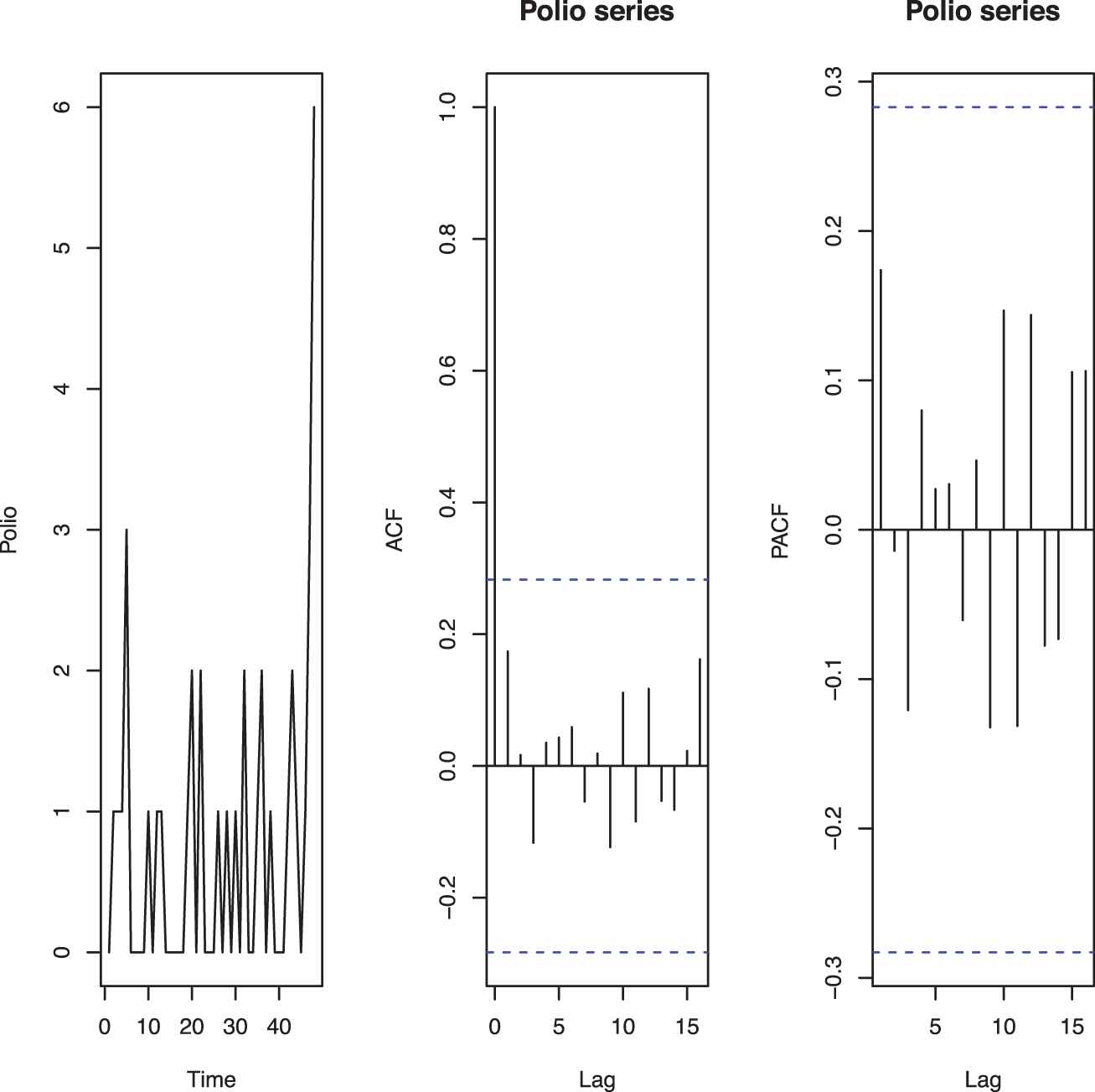
The sample path, Autocorrelation function (ACF) and Partial autocorrelation functions (PACF) plots of the number of polio cases, monthly from Jan 1980 to Dec 1983 in the United States.
| Model | YW Estimates |
RMS | ||
|---|---|---|---|---|
| PINMAP(1) | 1.156 | |||
| PINMAG(1) | 1.085 | |||
| PINMA(1) | 1.175 | |||
| GINMA(1) | 1.103 | |||
| NBINMAP(1) | 1.112 | |||
| NBINMAG(1) | 1.183 | |||
RMS, root mean square; PINMAP(1), first-order nonnegative integer-valued moving average process with power series innovations based on a Poisson thinning operator; YW, Yule-Walker
YW estimates of the parameters and RMS for the polio series.
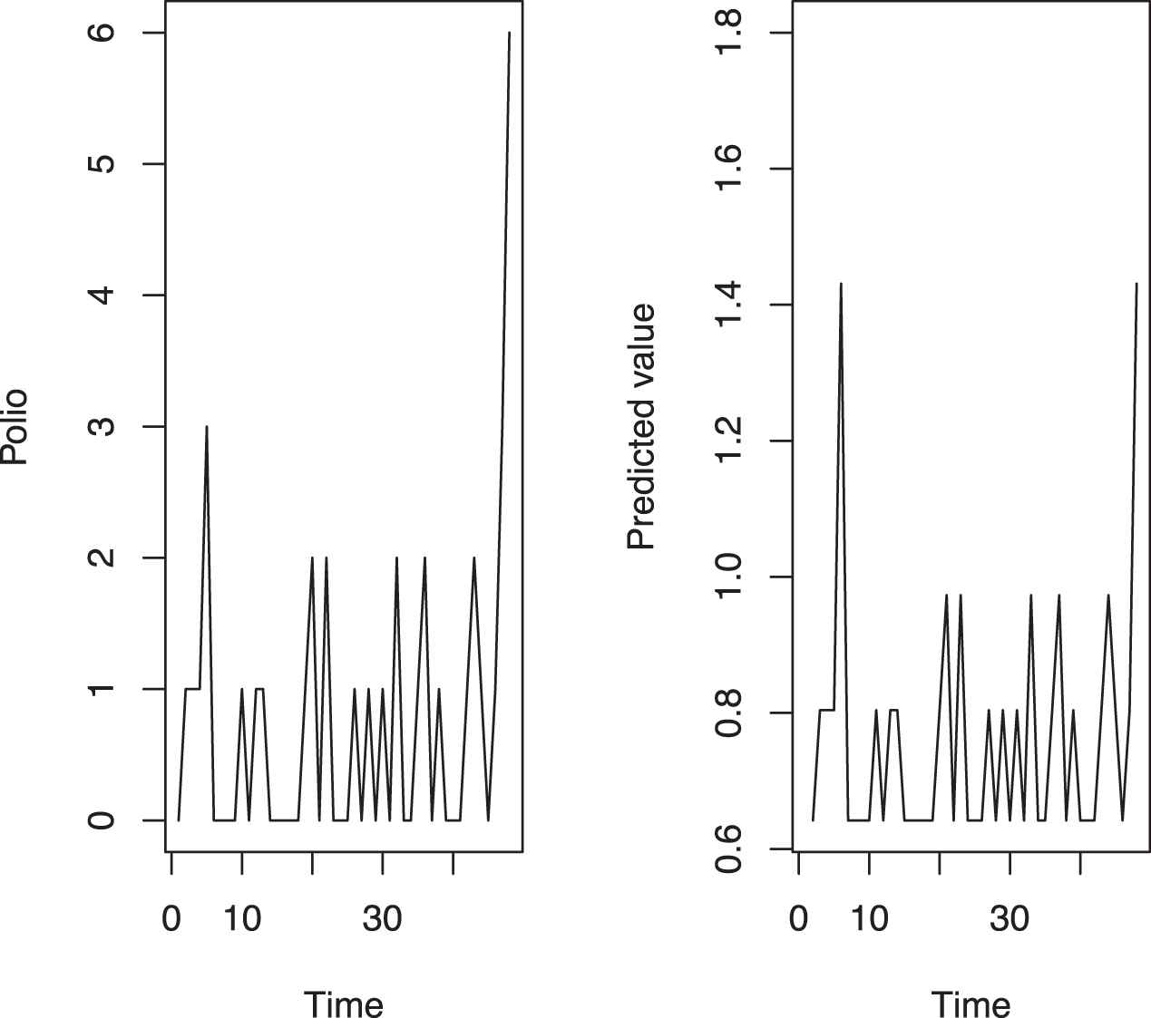
Polio data and their predicted values.
6.2. Number of Rubella Cases
The second example assumes the number of rubella cases, monthly from Jan 2013 to Jul 2017 in Spain (https://www.ecdc.europa.eu/sites/portal/files/media/en/publications/Publications/measles-rubella-monitoring-jan-(2013-2018).pdf). The sample path, autocorrelation and partial autocorrelation functions are shown in Figure 3. According to Figure 3, we observe that an INMA(1) process can be appropriate for modeling the rubella series since there exists a cut-off after lag 1 in the sample autocorrelation. The sample mean, variance and empirical index of dispersion are, respectively, 0.291, 0.321 and 1.104. Since the index of dispersion exceeds 1, the rubella series is overdispersed. Thus, the series must be modeled by an overdispersed model. We fit the PINMAP(1), PINMAG(1), PINMA(1), GINMA(1), NBINMAP(1) and NBINMAG(1) models to this data set. For each model, we obtain the YW estimates of the unknown parameters and RMS. The results are reported in Table 6. As we can see from Table 6, the PINMAP(1) has the lowest RMS compared to the other models, which indicates that the PINMAP(1) provides the best forecasting for the rubella series. Figure 4 shows the plots of the rubella data series and their predicted values based on the PINMAP(1) model.
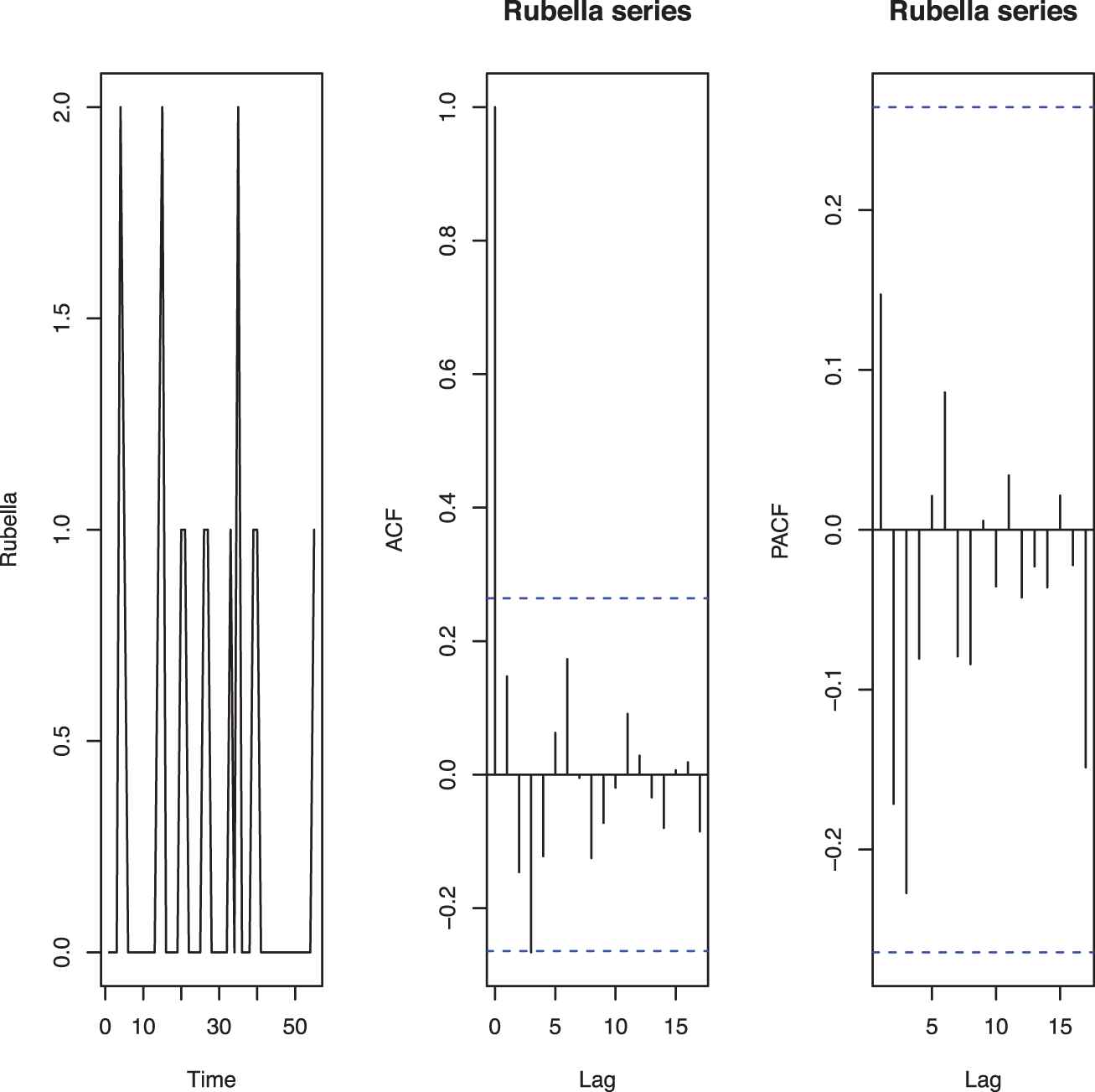
The sample path, ACF and PACF plots of the number of rubella cases, monthly from Jan 2013 to Jul 2017 in Spain.
| Model | YW Estimates |
RMS | ||
|---|---|---|---|---|
| PINMAP(1) | 0.5586 | |||
| PINMAG(1) | 0.5588 | |||
| PINMA(1) | 0.5595 | |||
| GINMA(1) | 0.5594 | |||
| NBINMAP(1) | 0.5663 | |||
| NBINMAG(1) | 0.6111 | |||
RMS, root mean square; PINMAP(1), first-order nonnegative integer-valued moving average process with power series innovations based on a Poisson thinning operator; YW, Yule-Walker
YW estimates of the parameters and RMS for the rubella series.
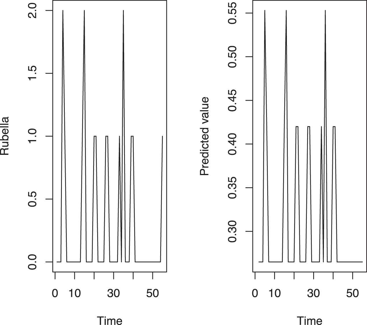
Rubella data and their predicted values.
6.3. Number of Earthquakes Magnitude 8.0 to 9.9
The third example assumes the number of earthquakes magnitude 8.0 to 9.9, annually from 1977 to 2006 in the world (http://www.johnstonsarchive.net/other/quake1.html). The sample path, autocorrelation and partial autocorrelation functions are shown in Figure 5. According to Figure 5, we observe that an INMA(1) process can be suitable for modeling this data set since there exists a cut-off after lag 1 in the sample autocorrelation. The sample mean, variance and empirical index of dispersion are, respectively, 0.67, 0.57 and 0.86. Since the index of dispersion lower than 1, the earthquakes series is underdispersed. Thus, an underdispersed model must be assumed for modeling the series. So we fit the PINMABE(1) and NBINMABE(1) models to this data set. For both models, we obtain the YW estimates and RMS. The results are shown in Table 7. According to the values of Table 7, we conclude that the PINMABE(1) model gives better forecasting than the NBINMABE(1) model for the earthquakes series because its RMS is smaller. Figure 6 shows the plots of the earthquakes data series and their predicted values based on the PINMABE(1) model.
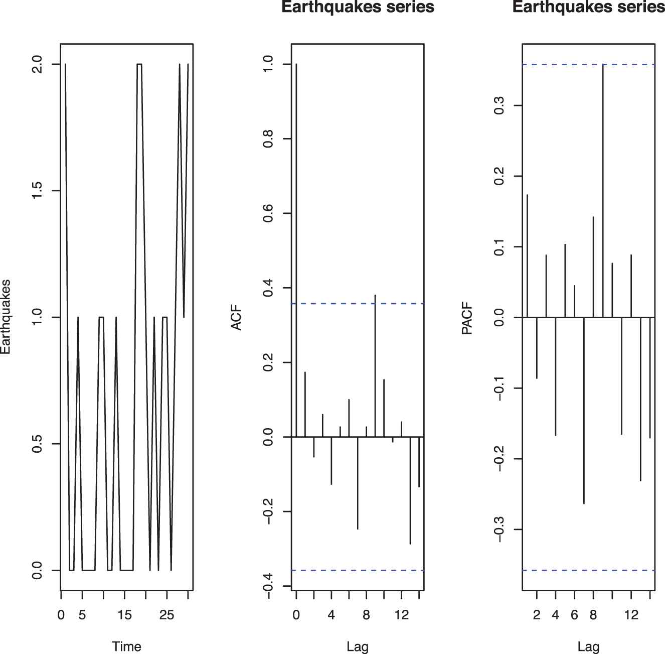
The sample path, ACF and PACF plots of the number of earthquakes magnitude 8.0 to 9.9, annually from 1977 to 2006 in the world.
| Model | YW Estimates |
RMS | |
|---|---|---|---|
| PINMABE(1) | 0.704 | ||
| NBINMABE(1) | 0.719 | ||
RMS, root mean square; YW, Yule-Walker
YW estimates of the parameters and RMS for the earthquakes series.
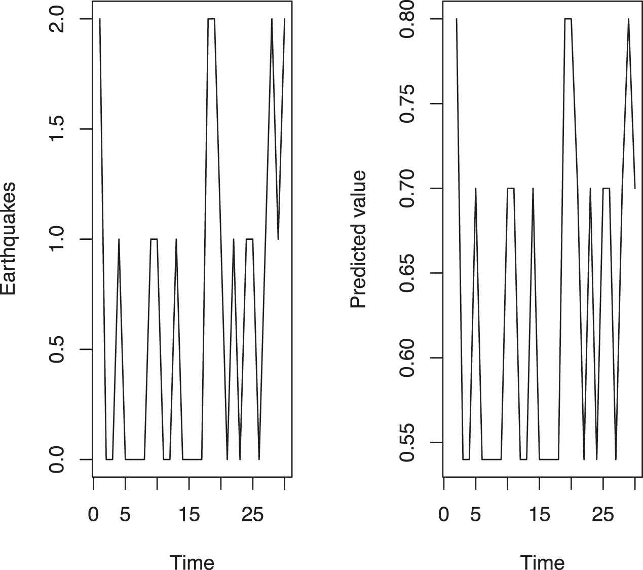
Earthquakes data and their predicted values.
7. CONCLUSION
In this paper, we consider a PINMAPS(1). Some statistical properties of the process are obtained. The stationary and ergodicity of the process are investigated. The parameters of the model are estimated using three methods contain YW, CLS and FGLS; also their performance is evaluated via simulation. Some sub-models are studied in detail. Finally, the model is applied to three real data sets and is shown the better performance of the model for predicting future values of overdispersed and underdispersed count data.
CONFLICTS OF INTEREST
There is no conflict of interest in this article.
AUTHORS' CONTRIBUTIONS
Mrs Rostami is the phd student under supervision of Prof. Eisa Mahmoudi and this work is related to her thesis.
ACKNOWLEDGMENTS
The authors thank the anonymous referees for their valuable comments and careful reading, which led to an improvement of the presentation and results of the article. The authors are grateful to the Editor-in-Chief and Editor for their helpful remarks on improving this manuscript. The authors are also indebted to Yazd University for supporting this research.
REFERENCES
Cite this article
TY  - JOUR
AU  - Eisa Mahmoudi
AU  - Ameneh Rostami
PY  - 2020
DA  - 2020/09/28
TI  - First-Order Integer-Valued Moving Average Process with Power Series Innovations
JO  - Journal of Statistical Theory and Applications
SP  - 415
EP  - 431
VL  - 19
IS  - 3
SN  - 2214-1766
UR  - https://doi.org/10.2991/jsta.d.200917.001
DO  - 10.2991/jsta.d.200917.001
ID  - Mahmoudi2020
ER  -