
New Discrete Lifetime Distribution with Applications to Count Data
- DOI
- 10.2991/jsta.d.210203.001How to use a DOI?
- Keywords
- Generalized Hermite distribution; Hermite polynomials; Genocchi polynomials; Hermite–Genocchi polynomials; Discrete distribution; Reliability
- Abstract
In this paper, we present a new class of distribution called generalized Hermite–Genocchi distribution (GHGD). This model is obtained by compounding generalized Hermite–Genocchi polynomials given by Gould and Hopper with powers series distribution. Statistical properties and reliability characteristics are studied. The model has been applied to several real data. Finally, a simulation study is performed to assess the performance of the model.
- Copyright
- © 2021 The Authors. Published by Atlantis Press B.V.
- Open Access
- This is an open access article distributed under the CC BY-NC 4.0 license (http://creativecommons.org/licenses/by-nc/4.0/).
1. INTRODUCTION
In this paper, we introduced a new discrete distribution based on the generalized Hermite polynomials given by, see [1]
Gupta and Jain [5] extended the Hermite distribution (HD) of the generalized HD defined by
The distribution has been applied to the frequency of bacteria in leucoytes and frequency of larvae in corn plants [6].
Moreover, there are a lot of popular statistical distributions that have specific applications, but sometimes, observable data contain distinct features not shown by these classic distributions. So to overcome these limitations, researchers often develop new distributions so that these new distributions can be used in these cases where the classical distributions don't provide any suitable fit. There are many techniques with which we can get new distribution, for more details see [7–9].
Recently, El-Desouky et al. [10] introduced a new generalized Hermite–Genocchi distribution (GHGD). By compounding (1) and powers series distribution defined new multivariate distribution called GHGD.
The paper is organized as follows: In Section 2, when set
2. GENERALIZED HERMITE–GENOCCHI DISTRIBUTION
Definition 2.1.
A discrete random variable
2.1. Structural Properties of GHGD Model
2.1.1. Shape and behavior of pmf plots of GHG distribution with serval values of parameters α , β γ
Three examples in Figure 1 showing effects of scale and shape parameters.
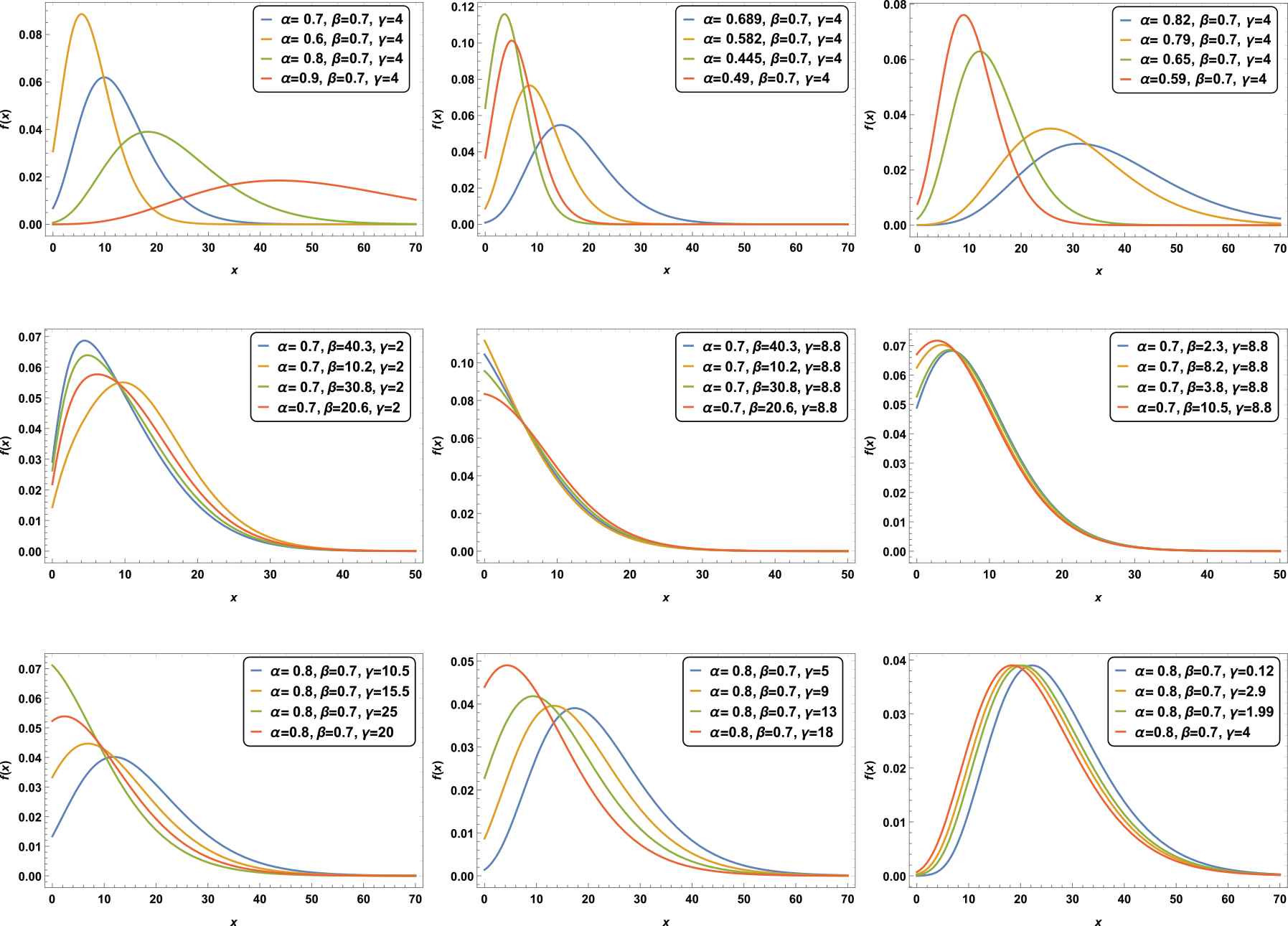
Shape and behavior of pmf plots of GHGD with serval values of parameters
2.1.2. Cumulative distribution function
The cumulative distribution function (cdf) of GHGD is given by
Figure 2 showing shape and behavior of Cdf plots of GHG distribution with several values of parameters α, β and γ.
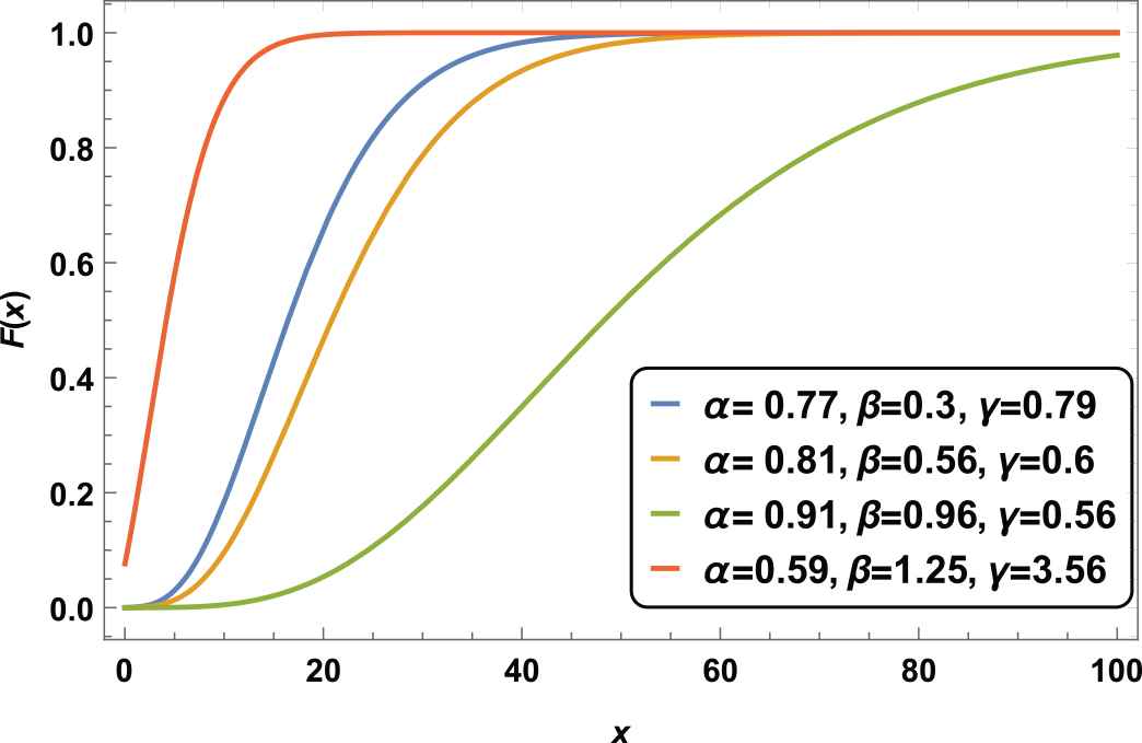
Cdf of GHGD for different values of
2.1.3. Moments and related measures
The moment-generating function of GHGD is given by
The
The
The mean and variance are given, respectively, by
The plots in Figure 3, it is apparent that both mean and variance of GHGD have bounds.
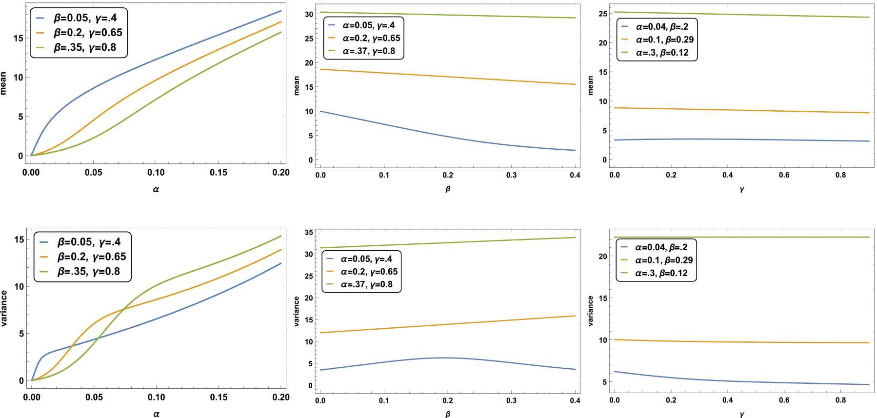
Plots the mean and variance of GHGD with serval values of parameters
2.1.4. Over-dispersion
The over-dispersion (OD) index of GHGD is given by
From Figure 3 and Eq. (2.2), we can obtain the following corollary:
Corollary 2.2.
OD
GHGD is no over-dispersion, over-dispersion and under-dispersion for
We obtained that numerically.
2.1.5. Surprise index
The surprise index (SI) of GHGD is given by
From Figure 4 for various value of
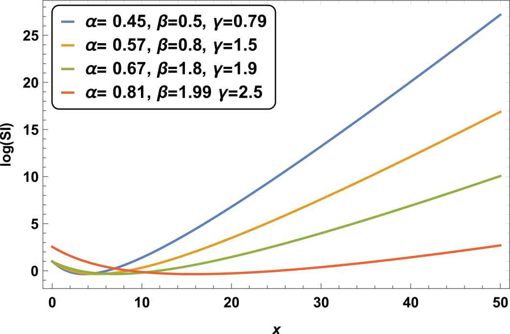
log(SI)'s for GHGD.
2.1.6. Generating function
The probability-generating function of GHGD is given by
3. MONOTONIC PROPERTIES
Log-concavity is an essential property of the probability distribution. Characteristics such as reliability function, failure rate, mean residual and moment of log-concave probability have specific properties see [11–14].
Theorem 3.1.
The GHG distribution is log-concave.
Proof.
Consider the function
Its derivative is given by
Note that
Corollary 3.2.
As a direct consequence of log-concavity, see [11], the following results hold for GHG distribution:
It is strongly unimodal.
It has all moments.
It has an increasing failure rate distribution.
It has monotonically decreasing mean residual function.
It remains log-concave if truncated.
It gives unimodal and log-concave distribution when convoluted with any other discrete distribution.
4. RELIABILITY PROPERTIES
The survival function of GHGD is given by
In Figure 5, shape and behaviour of survival function plots of GHG distribution with several values of parameters α, β and γ.
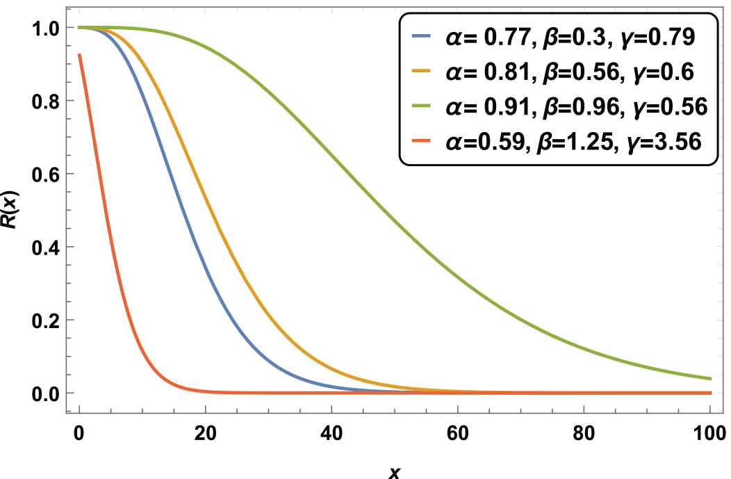
Survival function for GHGD.
Also, the hazard rate function is given by
The failure rate is increasing, see (Theorem 3.1) and (Corollary 3.2) and Figure 6.
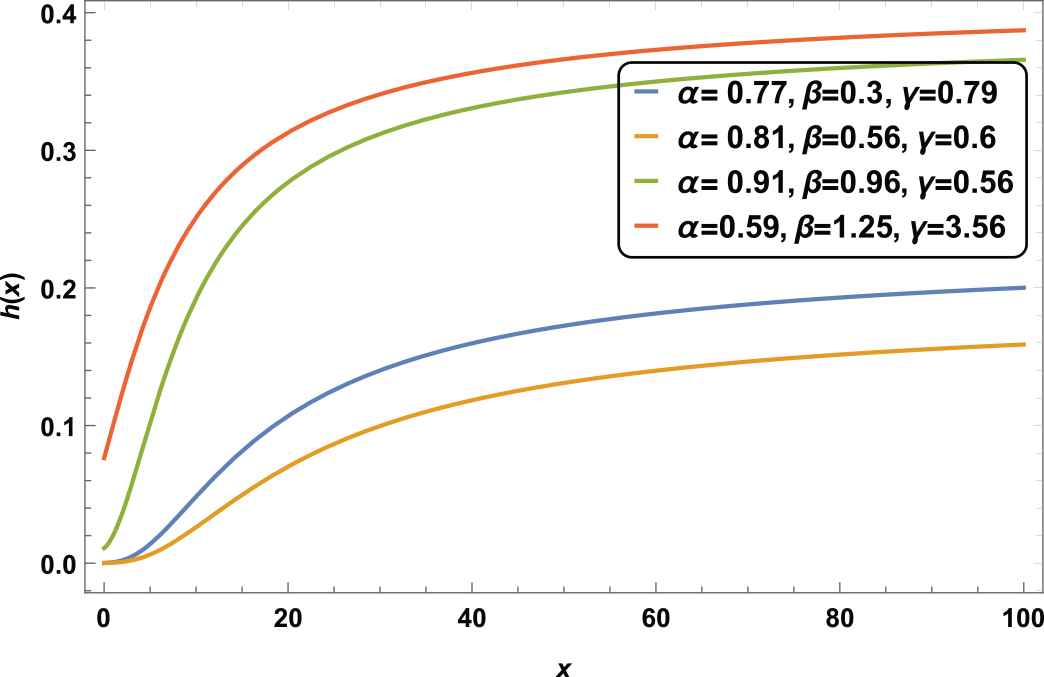
Hazard function for GHGD.
The mean residual life (MRL) of the GHGD is given by
The mean time to failure (MTTF) of GHGD is given by
The reversed hazard rate is given by
The shape and behavior of reversed hazard rate GHG distribution with several values of parameters α, β and γ, see Figure 7.
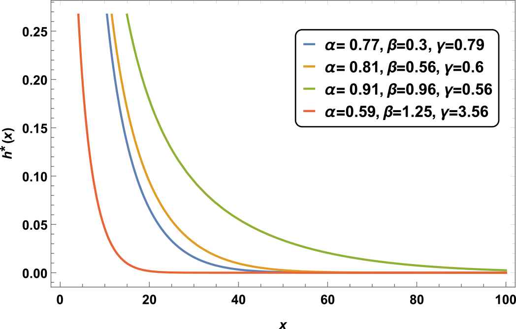
Reversed hazard function for GHGD.
Definition 4.1. [13]
A discrete distribution of nonnegative random variable is said to be
New better (worse) than used, denoted by NBU(NWU) if
New better (worse) than used in expectation, denoted by NBUE(NWUE) if
Corollary 4.2.
As a result of IFR, see [13], the following results hold:
GHGD is IFRA
GHGD is NBU
GHGD is DMRL
GHGD is NBUE.
5. PARAMETER ESTIMATION AND SIMULATION
5.1. Maximum Likelihood Estimators
Let
The log-likelihood function can be written as
Computing the first partial derivatives of (5.1) with respect to
Equating the Equations (5.2–5.4) to zero and solving them with the help of R software, the MLES can be obtained. We notice that, these equations cannot solve analytically, there is an alternative procedure like Newton-Raphson is required to solve them numerically.
5.2. Simulation
In this section, we evaluate MLE performance to sample
Generate
Calculate MLES for
Calculating absolute bias, standard errors and mean square errors (MSE).
The results obtained in Table 1.
| n | Parameter | MLE | Standard Error | Abs. Bias | MSE |
|---|---|---|---|---|---|
| 50 | 0.2187 | 0.011 | 0.0187 | 0.0005 | |
| 0.0809 | 0.057 | 0.0309 | 0.0038 | ||
| 0.2462 | 0.1434 | 0.0538 | 0.0212 | ||
| 100 | 0.2118 | 0.0137 | 0.0118 | 0.0003 | |
| 0.0573 | 0.018 | 0.0073 | 0.0003 | ||
| 0.3169 | 0.123 | 0.0169 | 0.0124 | ||
| 500 | 0.2086 | 0.0063 | 0.0086 | 0.0001 | |
| 0.0447 | 0.0069 | 0.0053 | 0.00007 | ||
| 0.2947 | 0.0414 | 0.0053 | 0.0017 | ||
| 800 | 0.2079 | 0.0059 | 0.0079 | 0.00009 | |
| 0.0455 | 0.004 | 0.0045 | 0.00004 | ||
| 0.3051 | 0.0408 | 0.0051 | 0.0016 | ||
| 1000 | 0.2065 | 0.0056 | 0.0065 | 0.00007 | |
| 0.0456 | 0.0045 | 0.0044 | 0.000039 | ||
| 0.3003 | 0.0348 | 0.0003 | 0.00121 |
Result from the simulated data.
It can be seen that
The bias values decrease as
MSEs decrease as
The MLE method performs well for the parameters.
6. DATA ANALYSIS
In this section, we explain the empirical importance of GHGD using real data applications. The fitted model is compared using
6.1. Data Set 1
This data represents counts of cysts in embryonic mouse kidneys which subjected to steroids, taken from McElduff et al. [15] and [16]. We compare the fits of GHGD with HD, zero-inflated Poisson distribution (ZIPD), negative binomial distribution (NBD), zero-inflated negative binomial distribution (ZINBD), zero-inflated generalized Poisson distribution (ZIGPD) and zero-inflated Hermite distribution (ZIHD). The MLES and goodness of fit are presented in Table 2.
| Count | Observed Frequency | HD | ZIPD | NBD | ZIGPD | ZINBD | ZIGH | GHGD |
|---|---|---|---|---|---|---|---|---|
| 0 | 65 | 17.938 | 60.87 | 20.87 | 85.113 | 63.7 | 65.02 | 64.86 |
| 1 | 14 | 24 | 3.5 | 24.6 | 8.64 | 5.5 | 11 | 14.16 |
| 2 | 10 | 24 | 7.5 | 20.973 | 6.307 | 6.02 | 9 | 7 |
| 3 | 6 | 19 | 9.5 | 15.57 | 5.9 | 6.2 | 8 | 6.52 |
| 4 | 4 | 12 | 9.6 | 10.71 | 4.99 | 5 | 5.5 | 5.36 |
| 5 | 2 | 6.77 | 7.8 | 7.02 | 0.05 | 6 | 2.5 | 3.9 |
| 6 | 2 | 3.3 | 5.44 | 4.449 | 4.2 | 2.52 | 2.77 | |
| 7 | 2 | 1.48 | 3 | 2.74 | 3.17 | 2.05 | 1.97 | |
| 8 | 1 | 0.612 | 1.5 | 1.7 | 2.27 | 0.9 | 1.4 | |
| 9 | 1 | 0.5 | 1.02 | 1.25 | 1.5 | 0.61 | 0.98 | |
| 10 | 1 | 0.5 | 0.27 | 0.58 | 3.04 | 0.6 | 0.68 | |
| 11 | 2 | 0.7 | 0.7 | 0.34 | 2.5 | 1.7 | 0.48 | |
| 12 | 1 | 0.2 | 0.5 | 0.198 | 1.9 | 1.6 | 0.92 | |
| Total | 111 | 111 | 111 | 111 | 111 | 111 | 111 | 111 |
| df | 4 | 5 | 4 | 1 | 4 | 3 | 2 | |
| Estimates of the parameter | ||||||||
| 154.39 | 27.66 | 117.43 | 34.07 | 22.62 | 2.32 | 1.77 | ||
| P value | 0.0001 | 0.0001 | 0.0001 | 0.0001 | 0.0001 | 0.0914 | 0.8804 | |
| AIC | 476.238 | 383.634 | 450.82 | 3238.76 | 371.02 | 368.4 | 353.287 | |
| BIC | 477.368 | 384.7 | 451.95 | 3240.45 | 372.71 | 370.24 | 361.415 | |
| AICc | 473.83 | 384.83 | 448.42 | 3236.09 | 368.35 | 365.22 | 353.511 |
Distribution of the counts of cysts from 111 steroid-treated kidneys [15] and the expected frequencies computed using HD, ZIPD, NBD, ZIGPD, ZINBD, ZIHD and GHGD.
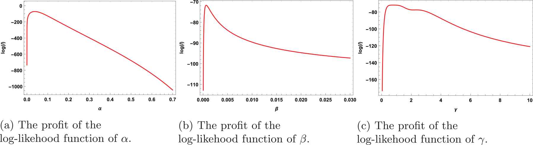
From the plots of the log-likelihood function of
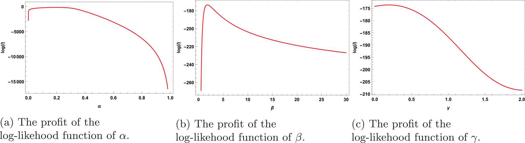
The profiles of the log-likelihood function of
6.2. Data Set 2
This data represents the distribution of mistakes in copying groups of random digits, see [17]. We compare the fits of GHGD with hyper-Poisson distribution (HPD), zero- inflated Poisson distribution (ZIPD), zero-inflated Conway–Maxwell–Poisson distribution (ZICMPD),ZINBD, ZIGPD and zero-inflated hyper-Poisson distribution (ZIHPD). The MLES and goodness of fit are presented in Table 3.
| Count | Observed Frequency | HPD | ZIPD | ZIHPD | ZICMPD | ZINBD | ZIGPD | GHGD |
|---|---|---|---|---|---|---|---|---|
| 0 | 35 | 24.41 | 41.1937 | 36.84 | 40.6 | 43.69 | 41.999 | 34.67 |
| 1 | 11 | 21.09 | 9.039 | 7.5 | 5.4 | 8.74 | 7.98 | 10.5 |
| 2 | 8 | 9.69 | 6.24 | 8.5 | 5.7 | 5.5 | 7.981 | 8.5 |
| 3 | 4 | 3.07 | 3.018 | 5.01 | 5.1 | 1.51 | 1.98 | 4.59 |
| 4 | 2 | 0.74 | 0.05093 | 2.05 | 3.2 | 0.56 | 0.06 | 1.74 |
| Total | 60 | 60 | 60 | 60 | 60 | 60 | 60 | 60 |
| df | 1 | 1 | 1 | 1 | 1 | 1 | 1 | |
| Estimates of the parameter | ||||||||
| 11.168 | 6.53 | 1.968 | 8.09 | 11.25 | 67.07 | 0.074 | ||
| P value | 0.0008 | 0.0106 | 0.1607 | 0.051 | 0.0008 | 0.0001 | 0.9948 | |
| AIC | 224.34 | 181.87 | 169.233 | 206.22 | 206.244 | 301.45 | 149.57 | |
| BIC | 221.74 | 179.27 | 165.332 | 205.13 | 205.072 | 300.82 | 155.853 | |
| AICc | 223.746 | 181.272 | 170.033 | 224.30 | 230.24 | 325.45 | 149.998 |
Distribution of mistakes in copying groups of random digits [17] and the expected frequencies computed using HPd, ZIPD, ZIHPD, ZICMPD, ZINBD, ZIGPD and GHGD distribution.
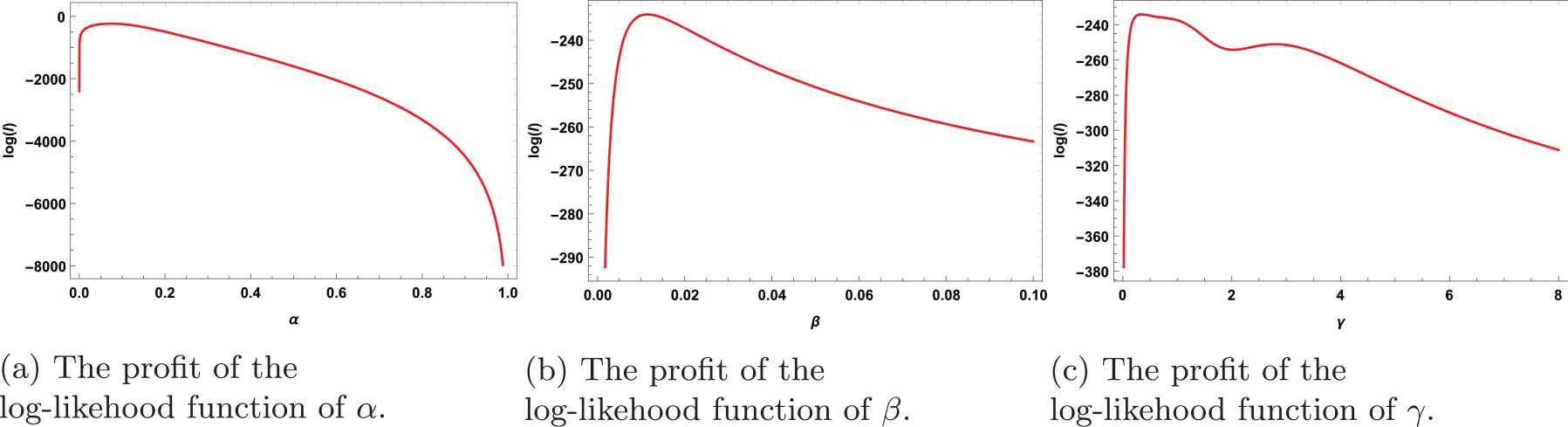
From the plots of the log-likelihood function of
The profiles of the log-likelihood function of
6.3. Data Set 3
This data represents counts of Collenbola microarthropods in 200 samples of forest soil, see [18,19]. We compare the fits of GHGD with (HPD), (ZIPD), (ZICMPD),(ZINBD), (ZIGPD) and (ZIHPD). The MLES and goodness of fit are presented in Table 4.
| Count | Observed Frequency | HPD | ZIPD | ZIHPD | ZICMPD | ZINBD | ZIGPD | GHGD |
|---|---|---|---|---|---|---|---|---|
| 0 | 122 | 135.133 | 134.46 | 118.5 | 129.6 | 133.79 | 157.33 | 120.09 |
| 1 | 40 | 54 | 28.7 | 36.56 | 40 | 41.2 | 25.75 | 39.85 |
| 2 | 14 | 7.31 | 21.1 | 23.24 | 24 | 17.2 | 9.5 | 18.52 |
| 3 | 16 | 1.58 | 11.05 | 14.25 | 5.2 | 5.61 | 5.5 | 13.07 |
| 4 | 4 | 1.5 | 3.64 | 5.5 | 0.5 | 1.72 | 1.35 | 5.97 |
| 5 | 2 | 0.74 | 1.05 | 1.95 | 0.8 | 0.48 | 0.57 | 2.5 |
| Total | 200 | 200 | 200 | 200 | 200 | 200 | 200 | 200 |
| df | 1 | 2 | 2 | 1 | 1 | 1 | 2 | |
| Estimates of the parameter | ||||||||
| 158.27 | 12.6 | 4.36 | 90.07 | 36.37 | 57.60 | 1.817 | ||
| P value | 0.0001 | 0.0018 | 0.1130 | 0.0001 | 0.0001 | 0.0001 | 0.7694 | |
| AIC | 1228.03 | 621.6 | 582.99 | 744.7 | 660.2 | 1298.1 | 474.151 | |
| BIC | 1227.6 | 621.18 | 582.37 | 744.15 | 659.5 | 1297.5 | 484.046 | |
| AICc | 1229.3 | 625.6 | 591.9 | 750.77 | 669.2 | 1307.1 | 474.273 |
Distribution of the counts of Collenbola microarthropods in 200 samples of fort soil [19] and the expected frequencies computed using HPD, ZIPD, ZIHPD, ZICMPD, ZINBD, ZIGPD and GHGD distribution.
From the plots of the log-likelihood function of
The profiles of the log-likelihood function of
6.4. Graphical Assesment of Goodness of Fit
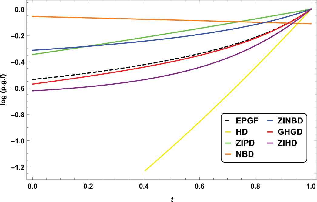
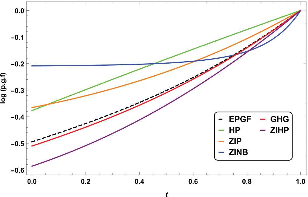
Plotting both the empirical probability generating function (EPGF) and log pgf's on the same graph allows us to compare the fit of a number of discrete distributions using only one plot, see [20].
The log of the EPGF of data set 1 is plotted in Figure 11. The EPGF is shown as black line, whilst a series of distributions fitted to data. The GHGD
EPGF plot of counts of cysts from 111 steroid-treated kidneys with fitted it log pgf's for the Hermite distribution, zero-inated Poisson distribution, negative binomial distribution, zero-inated negative binomial distribution and generalized Hermite–Genocchi distribution.
The log of the EPGF of data set 2 is plotted in Figure 12. The EPGF is shown as black line, whilst a series of distributions fitted to data. The GHGD

EPGF plot of the distribution of mistakes in copying groups of random digits with fitted it log pgf's for the hyper-Poisson distribution, zero-inflated Poisson distribution, zero-inflated negative binomial distribution, zero-inflated hyper-Poisson distribution and generalized Hermite–Genocchi distribution.
The log of the EPGF of data set 3 is plotted in Figure 13. The EPGF is shown as black line, whilst a series of distributions fitted to data. The GHGD
EPGF plot of counts of Collenbola microarthropods of forest soil with fitted it log pgf's for the hyper-Poisson distribution, zero-inflated Poisson distribution, zero-inflated negative binomial distribution, zero-inflated hyper-Poisson distribution and generalized Hermite–Genocchi distribution.
7. CONCLUSION
A new three parameters discrete distribution is proposed and its important monotonic and reliability concepts are introduced. The model proposed parameters are estimated by Maximum likelihood and the simulation study is performed to establish the accuracy of the maximum likelihood estimators. Applications of the new model in the analysis of three real-life data are presented. We show by three applications of the real data that the proposed distribution can yield better fits than some other distributions.
CONFLICTS OF INTEREST
The authors declare they have no conflicts of interest.
AUTHORS' CONTRIBUTIONS
All authors have read and agreed to the published version of the manuscript.
ACKNOWLEDGMENTS
The author would like to thank the Editor-in-Chief, and the anonymous referees for their careful reading and constructive comments and suggestions which greatly improved the presentation of the paper.
REFERENCES
Cite this article
TY  - JOUR
AU  - Beih S. El-Desouky
AU  - Rabab S. Gomaa
AU  - Alia M. Magar
PY  - 2021
DA  - 2021/02/22
TI  - New Discrete Lifetime Distribution with Applications to Count Data
JO  - Journal of Statistical Theory and Applications
SP  - 304
EP  - 317
VL  - 20
IS  - 2
SN  - 2214-1766
UR  - https://doi.org/10.2991/jsta.d.210203.001
DO  - 10.2991/jsta.d.210203.001
ID  - El-Desouky2021
ER  -