
The XLindley Distribution: Properties and Application
- DOI
- 10.2991/jsta.d.210607.001How to use a DOI?
- Keywords
- Exponential distribution; Lindley distribution; quantile function; method of moment; maximum likelihood method; simulation
- Abstract
This paper proposes a new distribution called XLindley distribution (XLD), this distribution is generated as a special mixture of two distributions: exponential and Lindley and hence the name proposed. Also, the statistical properties like stochastic ordering, quantile function, the maximum likelihood method and method of moments. An application of the model to a real data set presented finally and compared with the fit and shows that XLD has more flexibility than others one-parameter distributions.
- Copyright
- © 2021 The Authors. Published by Atlantis Press B.V.
- Open Access
- This is an open access article distributed under the CC BY-NC 4.0 license (http://creativecommons.org/licenses/by-nc/4.0/).
1. INTRODUCTION
The real-life applications of contemporary numerical techniques in different fields such as medicine, finance, biological engineering sciences and statistics. To this end, statistics plays a critical role in our real-life applications. Often by using the statistical analysis which strongly depends on the assumed probability model or distributions. However, several problems in statistics do not follow any of the classical or standard probability models.
Let X is a random variable following the one-parameter distribution with density function called Lindley (LD) distribution:
It has introduced by Lindley [1]. Sankaran [2] used (1) as mixing distribution of poisson parameter which it named poisson-LD distribution. Recently, Asgharzadeh et al. [3], Zeghdoudi and Nedjar [4], Zeghdoudi and Bouchahed [5], Beghriche and Zeghdoudi [6], Ghitany et al. [7,8] rediscovered and studies the distribution bounded to (1), what that derived is known as Zero-truncated poisson-LD and pareto poisson-LD distributions.
Recently, Zeghdoudi and Nedjar [9,10] introduced a new distribution named Gamma LD distribution based on mixture of gamma distribution with scale parameter
The idea of this work is based on special mixture of exponential and LD distributions in order to create the XLindley distribution (XLD). This work is motivated by the following: XLD it is simple and easy to apply; the formulas of the mean, variance, coefficient of variation, skewness, kurtosis and index of dispersion are simple in form and may be used as quick approximations in many cases. However, in general it is applicable to try out simpler distributions than more complicated ones; the XLD can be used quite effectively in analyzing many real lifetime data set: application to Ebola, Corona and Nipah virus and gives adequate fits too many data sets.
The paper is organized as follows: Section 2 is devoted to introduce the methodology and gives survivals properties of XLD. Section 3 discusses the estimation of its parameter using method of moment and maximum likelihood. Finally, we present illustrative example of XLD with other distributions to show the superiority and flexibility of this model that found.
2. METHODOLOGY AND SURVIVAL PROPERTIES
In this section, a mixture of two known distributions used to give new distribution called XLD. Let X be a random variable following mixture distribution, it's density function (pdf)
With:
We consider
The first derivative of
gives:
For:
And the second derivative is:
Therefore, the mode of XL is given by:
We can find easily the cumulative distribution function (CDF) of the XLD:
The shapes of the PDF, CDF and hazard function of the XLD distribution are given in Figures 1–3 for different values of the parameter theta.
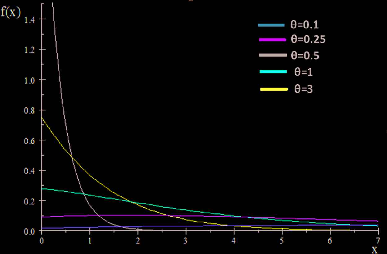
Plots of the density function for some parameter values
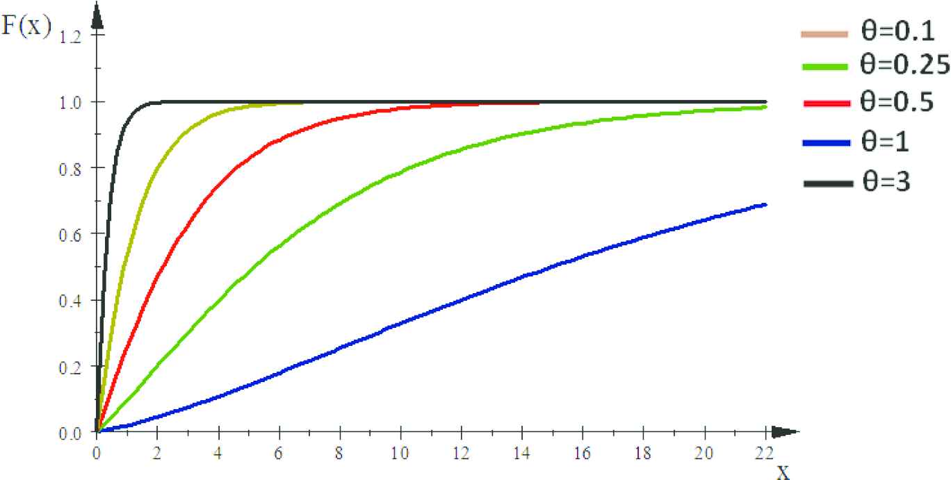
Plots of cumulative distribution function (CDF) for some parameter values
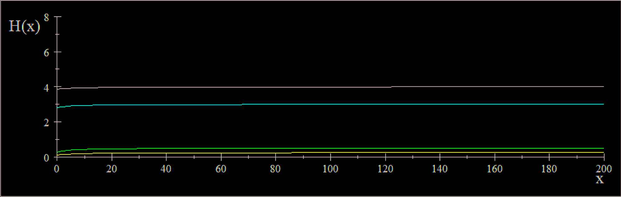
Plots of hazard function for some parameter values: blue (0.25); pink (0.5); red (3); black (4)
3. SURVIVAL AND HAZARD RATE FUNCTION
The survival function and failure rate (hazard rate) function for a continuous distribution are defined as:
Let:
and:
Proposition 1.
Let HXL (x) be the hazard rate function of X. Then HXL (x) is increasing.
4. MOMENTS AND RELATED MEASURES
The rth moment about the origin of the XLindey distribution can be obtained as:
Using gamma integral and little algebraic simplification, we get finally a general expression for the rth factoriel moment of XLD as:
Substituting r =1,2,3 and 4 in (9), the first four moments can be obtained and then using the relationship between moments about origin and moment about mean, the first four moment about origin of XLD were obtained as:
Proposition 2.
Let X ∼ XL(x), the mean, variance, coefficients of variation, skewness and kurtosis for X are:
Skewness, Kurtosis and Coefficient of variation of XLD:
The coefficients are increasing functions in θ (see Figure 4 for the graphe of C.V (γ) and Skewness
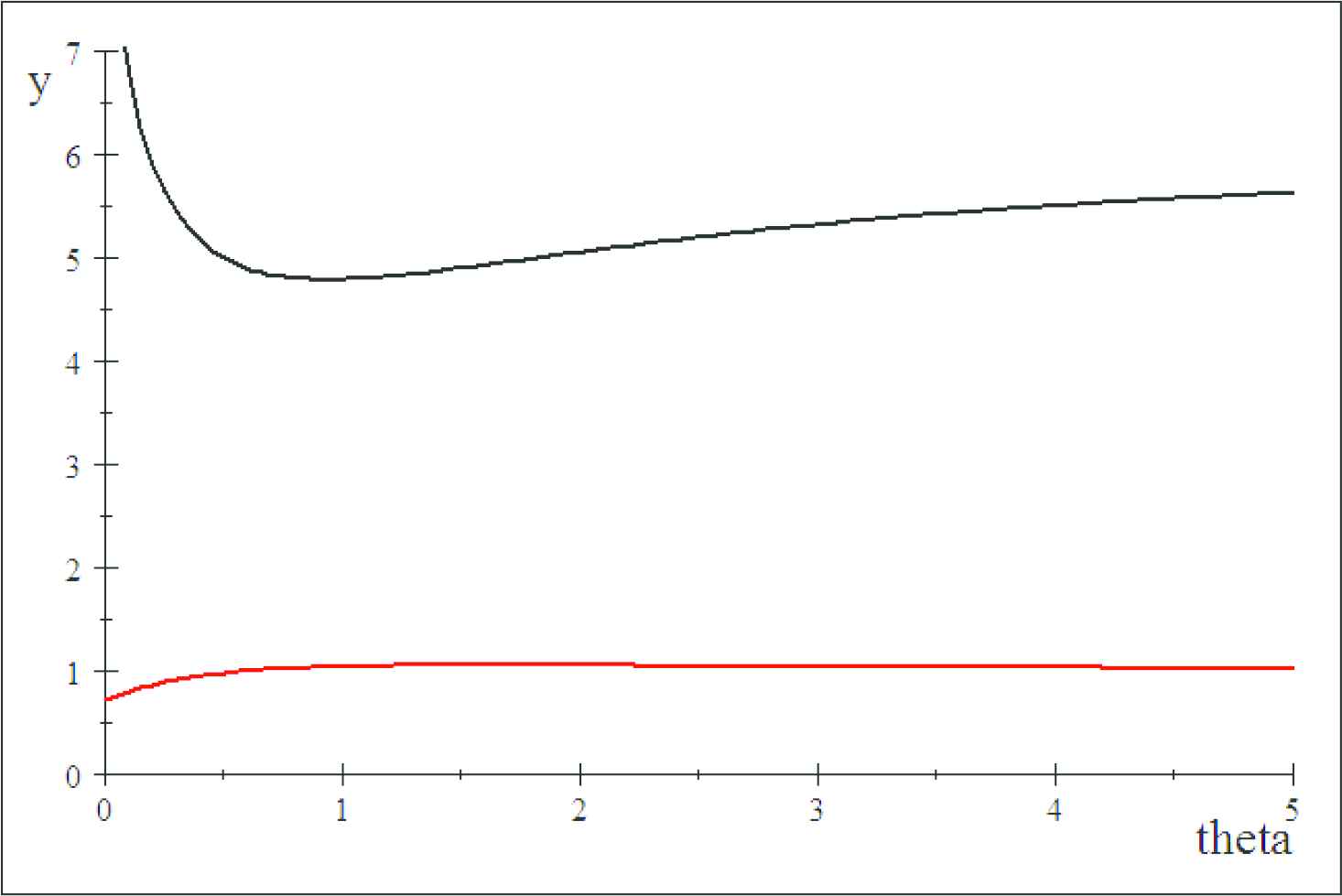
Coefficients for variation (red) and skewness (black)
5. STOCHASTIC ORDERING
Definition 1.
Consider two random variables
Stochastic order
Convex order
Hazard rate order
Likelihood ratio order
Remark 1.
Likelihood ratio order
Convex order
Theorem 1.
Let
Proof.
We have:
For simplification, we use
To this end, if
6. ESTIMATION OF PARAMETER
6.1. Method of Moments Estimation
Let
Putting the expression of E(x) from equation (10) in the equation and solving the equation for θ, We get:
We obtain equation of 3rd degree:
6.2. Maximum Likelihood Estimation
Let
Logarithm of likelihood function is:
The derivative of
To obtain the maximum likelihood estimation (MLE) of
The following theorem shows that the estimator of
Theorem 2.
the estimator
Proof.
Let
Finally, since
7. THE QUANTILE FUNCTION OF XLD
It may be noted that FX(x) in equation (5) is continues and strictly increasing, so we for the quantile function of X is defined:
For
Theorem 4.
For any
Where
Proof.
For any
We multiplying the both sides by
By using the definition of Lambert W function
So, we have
In addition to that, for any
This in turn means the result that given before in Theorem 4 is complete.
8. SIMULATION
We can see that the equation
In this subsection, we investigate the behavior of the ML estimators for a finite sample size (n). A simulation study consisting of the following steps is being carried out N = 10000 times for selected values of
- –
Generate
- –
Generate
- –
Generate
- –
If
The result of the simulation is presented in Tables 1 and 2. The following observations are made from the simulation study:
For some given value of
The mean square error (MSE) gets higher and following a similar ways for larger value of
| Bias | |||||
|---|---|---|---|---|---|
| 0.0032 | 0.01067 | 0.0485 | 0.276 | 0.785 | |
| 0.00183 | 0.0150 | 0.0135 | 0.126 | 0.1770 | |
| 0.000321 | 0.00404 | 0.0147 | 0.0452 | 0.0598 |
MSE, mean square error.
Average bias of the estimator
| MSE | |||||
|---|---|---|---|---|---|
| 1,0854.10-5 | 0.000113 | 0.00236 | 0.0765 | 0.6177 | |
| 3,357.10-6 | 0.000225 | 0.000183 | 0.01599 | 0.03135 | |
| 1,0334.10-7 | 1,640.10-5 | 0.000217 | 0.00204 | 0.00358 |
The average square error of the estimator
9. APPLICATION AND GOODNESS OF FIT
Now we have used data of survival times (in months) of 94 sierra leone individus infected with Ebola virus showing in Table 3, which we compare LD, Zeghdoudi (ZD), see (Messaadia and Zeghdoudi [14]), Exponential, Xgamma see (Sen et al. [15]) and XLD.
| Survival Time m = 3.17 s = 2.095 | Obs freq | LD |
Xgamma |
ZD |
Exp |
XLD |
|---|---|---|---|---|---|---|
| [0,2] | 45 | 38. 262 | 37. 652 | 30. 339 | 43. 937 | 41. 028 |
| [2,4] | 22 | 28. 164 | 27. 197 | 37. 27 | 23. 4 | 25. 855 |
| [4,6] | 17 | 15. 075 | 16. 342 | 17. 743 | 12. 463 | 13. 984 |
| [6,8] | 7 | 7. 1187 | 7. 7769 | 6. 1658 | 6. 6375 | 6. 9986 |
| [8,10] | 3 | 3. 1423 | 3. 2015 | 1. 828 | 3. 5351 | 3. 3409 |
| Total | 94 | 94 | 94 | 94 | 94 | 94 |
| 2. 7899 | 3. 2040 | 14. 236 | 1. 8619 | 1. 6446 |
LD, Lindley; XLD, XLindley distribution; ZD, Zeghdoudi.
Comparison between LD, Xgamma, ZD, Exp and XLD.
10. CONCLUSION
In this work, we present a one-parameter distribution called XLD which is mixture of two known distribution Exponential
CONFLICTS OF INTEREST
The authors declare they have no conflicts of interest.
AUTHORS' CONTRIBUTIONS
Study conception and design: H. Zeghdoudi; analysis and interpretation of results: S. Chouia; draft manuscript preparation: S. Chouia and H. Zeghdoudi. All authors reviewed the results and approved the final version of the manuscript.
Funding Statement
This research was funded by PRFU Program of Ministry of Higher Education and Scientific Research No. C00L03UN230120180014.
ACKNOWLEDGMENTS
The authors acknowledge editor in chief, Prof. Dr. Mohammad Ahsanullah and the referee, of this journal for the constant encouragement to finalize the paper.
REFERENCES
Cite this article
TY  - JOUR
AU  - Sarra Chouia
AU  - Halim Zeghdoudi
PY  - 2021
DA  - 2021/07/10
TI  - The XLindley Distribution: Properties and Application
JO  - Journal of Statistical Theory and Applications
SP  - 318
EP  - 327
VL  - 20
IS  - 2
SN  - 2214-1766
UR  - https://doi.org/10.2991/jsta.d.210607.001
DO  - 10.2991/jsta.d.210607.001
ID  - Chouia2021
ER  -