Mixture copula; Farlie-Gumbel-Morgenstern copula; Negative quadrant; Dependency order statistics
Abstract
In this study a new mixture copula has been obtained by creating a linear combination of product copula with copula which is obtained with marginal distributions of order statistics which was proposed by Dolati and Úbeda-Flores, Kybernetika. 45 (2009), 992–1002. In addition, a new form of Farlie-Gumbel-Morgenstern copula is obtained by applying Farlie-Gumbel-Morgenstern copula to new mixture copula. The new form of the Farlie-Gumbel-Morgenstern copula has been compared to Farlie-Gumbel-Morgenstern, Gaussian and Frank copulas. To find the best-fit copula, Akaike information criterion and Bayesian information criterion are used.
Copulas are the special functions obtained with a combination of functions. Therefore, appropriate conversions can be made to create new copulas or to improve the existing copulas. Recently many researchers have aimed to obtain variables with higher correlation by improving the existing copulas or building new copulas. One of the most important parametric copula families, Farlie-Gumbel-Morgenstern (FGM) copula has drawn the attention of the researchers to a great extent due to its easy algebraic features. The biggest disadvantage of the FGM copula is that the lower and upper bounds of Spearman’s.. and Kendall’s τ are [−1/3,1/3] and [−2/9,2/9], respectively. Researchers have recommended new forms of FGM copula to widen this limited dependency. Huang and Kotz [1], Bairamov and Kotz [2], Lai and Xie [3], Bairamov et al. [4], Rodríguez-Lallena and Úbeda-Flores [5], have worked on several new modifications of the FGM family. Using the marginal distributions of order statistics, Dolati and Úbeda-Flores [6] obtained two new different copulas and examined the properties of the copulas. Also, they obtained two new forms of FGM copula by applying the obtained copulas to the FGM copula. Bayramoğlu and Bairamov [7] have formed a new bivariate variable distribution with high correlation based on distribution of the order statistics, by using a randomly selected continuous copula.
A new mixture copula has been obtained by creating a linear combination of the copula obtained from the marginal distributions of the order statistics proposed by Dolati and Úbeda-Flores [6] with the product copula. The ordering property, quadrant dependency, concordance, relations of the obtained new mixture copula to the known copulas and new bounds for Kendall’s τ and Spearman’s ρ has been obtained. In addition, the new mixture copula is applied to the FGM copula to obtain a new form of FGM copula. Then, the new form of the FGM copula is compared with copulas (FGM copula, Gaussian copula and Frank copula) appropriate to negative correlation with different alpha possibilities, without exceeding the parameter bounds with simulation study in detail. Here, in order to find the best-fit copula, Akaike information criteria and Bayesian information criteria have been used.
2. BASIC PROPERTIES OF COPULAS
A copula is a function C:0,12→0,1 which satisfies following properties:
The boundary conditions, for all u,v∈I:
Cu,0=C0,v=0.
Cu,1=u and C1,v=v.
The 2-increasing property, for every u1,u2,v1,v2∈I such that u1≤u2 and v1≤v2:C(u2,v2)−C(u2,v1)−C(u1,v2)+C(u1,v1)≥0, [8].
Following result is an important theory for copulas.
Theorem 1 (Sklar’s Theorem).
His a joint distribution function with marginsFandG. For everyx,y∈R¯we have
Hx,y=CFx,Gy,(1)
where C is a copula. If F and G are continuous, C is unique; otherwise, C is uniquely determined on RangeF×RangeG. Contrarily, if C is a copula and F and G are distribution functions, then the function H defined by (1) is a joint distribution function with margins F and G [9].
∏ denote the product copula and ∏u,v=u.v for every u,v∈0,12. Let X and Y are continuous random variables, if CX,Y=∏ then X and Y are independent.
For any copula C, Mu,v=minu,v is minimum copula and Wu,v=maxu+v−1,0 is maximum copula for all u,v∈I2. The following inequality is provided for all copulas:
Wu,v≤Cu,v≤Mu,v.
C^ denote the survival copula and C^:I2→I function is defined as follows:
C^u,v=u+v−1+C1−u,1−v.(2)
C¯ denote the survival function and is defined as follows:
C¯u,v=PU>u,V>v=1−u−v+Cu,v=C^1−u,1−v.(3)
In (2) and (3) equalities, C^ is always a copula but C¯ is a copula only if it provides boundary condition.
The probability density function of copulas can be obtained as follows [8]:
cu1,u2,...um=∂mCu1,u2,...um∂u1∂u2...∂um,(4)
2.1. Kendall’s τ and Spearman’s ρ
Kendall’s τ and Spearman’s ρ are nonparametric measures of association of between two random variables X and Y. The relations of Kendall’s τ and Spearman’s ρ with C copula is given by Theorems 2 and 3.
Theorem 2.
LetCis common copula of continuous random variablesXandY. Then Kendall’sτ is given as follows [8]:
τ(C)=4∫01∫01Cx,ydCx,y−1,(5)
Theorem 3.
LetCis common copula of continuous random variablesXandY. Then Spearman’sρis given as follows [8]:
ρC=12∫01∫01Cx,ydxdy−3,(6)
2.2. Archimedean Copulas
Archimedean copulas are widely using in applications because of they can be constructed easily and they have many nice algebraic properties.
2.2.1. Properties of Archimedean copulas
Let φ is a continuous, strictly decreasing function on φ:I→0,∞ such that φ1=0 and φ−1 is pseudo-inverse of φ and Domainφ−1=0,∞, Rangeφ−1=0,1 is given by
φ−1t=φ−1t,0≤t≤φ00,φ0≤t≤∞.(7)
Point out that φ−1 is a continuous and nonincreasing on 0,∞ and strictly decreasing on 0,φ0. Hence, C:0,12→0,1 is defined as follows:
Cu,v=φ−1φu+φv.(8)
This form (8) of copulas are called Archimedean copulas and φ is called a generator of the copula. If φ0=∞, φ is a strict generator and in this case, φ−1φu+φv is said to be a strict Archimedean copula. Properties of generators is given as below.
φ1=0.
For every t∈0,1, φ′t<0.
For every t∈0,1, φ″t≥0.
Theorem 4.
LetCis an Archimedean copula andφits generator:
Cis symmetric, namely, for everyu,v∈I,Cu,v=Cv,u.
Cis associative, namely, for everyu,v,w∈I,CCu,v,w=Cu,Cv,w.
Ifc>0is any constant,cφis also a generator ofC [8].
2.3. FGM Copula
FGM copula is an important copula family for researchers to a great extent due to its easy algebraic features. As a result of their work de la Horra and Fernandez [10] claimed that FGM family was a strong class among prime copula families. FGM copula is defined as follows:
Cθu,v=uv1+θ1−u1−v,θ∈−1,1(9)
The relations of Kendall’s τ and Spearman’s ρ with FGM are respectively τ=2θ9 and ρ=θ3 [8].
2.4. Gaussian Copula
The Gaussian copula is derived from multivariate Gaussian distribution. Φ is the distribution function of one-dimensional standart normal distribution and let ΦΣn is the distribution function of the positive definite correlation matrix Σ and n-dimensional standart normal distribution. Hence, n-dimensional Gaussian copula CΣΦ is defined as follows:
where ρ12 is the correlation coefficient of bivariate standart normal distribution. The relation of Kendall’s τ with Gaussian copula is defined as follows:
In this section, a new mixture copula has been obtained from Dolati ve Úbeda-Flores’s [6] study. The preliminary of their study is given as follows.
Let X1,Y1 and X2,Y2 be two independent vectors of uniform 0,1 random variables with common copula D. Let X1,X2 and Y1,Y2 be their corresponding order statistics. Consider the random vector:
For any D copula, a new bivariate distribution function CaΔD defined from 0,12→0,1 by
CaΔD=αDx,y−αDx,yD¯x,y+∏x,y−α∏x,y.(12)
where 0≤α≤1.
When we apply the new mixture copula to some important copulas, the following situations are achieved.
Situation 1. Consider the copula M. Since M¯x,y=M1−x,1−y for every x,y in 0,12we have Mx,yM¯x,y=Mx,y−∏x,y. Then we have
CaΔM=αMx,y−αMx,y+α∏x,y+∏x,y−α∏x,y=∏x,y.
Obtained copula is product copula.
Situation 2. Consider the copula W. Since Wx,yW¯x,y=0 for every x,y in 0,12, we have
CaΔW=αWx,y+1−α∏x,y.
Obtained copula is constitute of Fréchet-Mardia family of copulas.
Situation 3. Consider the product copula ∏. Then we have
CaΔ∏=αxy−αxy1−x1−y+xy−αxy=xy1−α1−x1−y.
Obtained copula is constitute of FGM family of copulas.
2.5.1. Some properties of the new mixture copula
Symmetry: A copula D is symmetric if Dx,y=Dy,x for all x,y∈0,1 [8].
Theorem 5.
If the copulaDis symmetric, thenCaΔDis symmetric as well.
Proof.
CaΔDy,x=αDy,x−αDy,xD¯y,x+∏y,x−α∏y,x.
Since Dx,y=Dy,x and D¯x,y=1−x−y+Dx,y, thus D¯y,x=1−x−y+Dy,x and D¯x,y=D¯y,x. On the other hand, since ∏x,y=x.y=y.x, we easily obtain CaΔDy,x=CaΔDx,y, which completes the proof.
Radially symmetry: A copula C is radially symmetric if C=C^, i.e., C(x,y)=x+y−1+C(1−x,1−y) [8].
Theorem 6.
If the copulaDis radially symmetric, thenCαΔDis radially symmetric for eachα∈0,1as well.
Here, we have D(1−x,1−y)=D^¯(x,y), D¯(1−x,1−y)=D^(x,y) and ∏(x,y)=∏^(x,y). Thus C^aΔ[D]=CaΔ[D^]=CaΔ[D], which completes the proof.
Order: A totally ordered parametric family {Cα} of copulas is positively ordered if Cα1<Cα2 whenever α1≤α2; and negatively ordered if Cα1>Cα2 whenever α1≤α2 [8].
Theorem 7.
The parametric familyCαΔ[D]of copulas is negatively ordered.
Proof.
CαΔ[D] is positively ordered if Cα1Δ[D](x,y)−Cα2Δ[D](x,y)<0 whenever α1≤α2 and negatively ordered if Cα1Δ[D](x,y)−Cα2Δ[D](x,y)>0 whenever α1≤α2. We have
Since x≥D1(x,y) and y≥D2(x,y), which completes the proof.
Theorem 10.
For a given copulaDand for eachα∈[0,1], new boundaries for Kendall’sτand Spearman’sρhave obtained as follows:
(−α)(α+2)3≤τCαΔ[D]≤0,
−α≤ρCαΔ[D]≤0.
Proof.
C1 and C2 are two copulas such that C1<cC2, we have τ(C1)≤τ(C2) ve ρ(C1)≤ρ(C2) [8]. Since any copula C satisfies that W(x,y)≤C(x,y)≤M(x,y) we have
αW(x,y)+(1−α)∏(x,y)<CαΔ[D](x,y)<∏(x,y). Here τ∏(x,y)=0. On the other hand, Fréchet-Mardia family of copulas which is usually written as Cα,β(x,y)=βM(x,y)+(1−α−β)∏(x,y)+αW(x,y), we have τα,β=(β−α)(α+β+2)3 and ρα,β=β−α [8]. Note that β=0 is taken here and then we can easily obtain the new boundaries. This completes the proof.
2.5.2. A new form of FGM copula
The new mixture copula is applied to FGM copula and a new form of FGM copula is obtained as follows:
For α∈[0,1] and θ∈[−1,1], we obtain ρCΔ[Dθ]∈−0.513^,0 and τCΔ[Dθ]∈[−0.3492517,0]. For (α,θ)=(1,−1), Kendall’s τ and Spearman’s ρ are decreased down to τ=−0.3492517 and ρ=−0.513^, respectively. Because of the new mixture copula is NQD, the new form of FGM copula have found stronger dependency on the negative side.
3. THE BEST-FİT COPULA
The new form of FGM copula is compared some copulas. The best-fit copula is identified by comparing the evaluated values of the Akaike Information Criterion- AIC [12] and Bayesian Information Criterion- BIC [13] which are defined as
AIC=−2∑i=1Nlncui,vi+2k,(14)
BIC=−2∑i=1Nlncui,vi+klnN,(15)
where k is the number of copula parameters, N is the sample size and c(ui,vi) is the probability density function of C(ui,vi). Let (X,Y) be measured data, ui,vi are rank of (X,Y) which are defined as
ui=rankXiN+1vi=rankYiN+1i=1,2,…,N(16)
where rank(Xi)(orrank(Yi)) denotes the rank of Xi(orYi) among X(orY) in an ascending order. Thus the measured data in original space is transformed into the standart uniform random vector (u,v) [14].
Copula density functions c(u,v), copula parameter (ρ12 and θ) intervals and connecting with Kendall’s τ are given in Table 1.
Since the new form of FGM copula is appropriate to negative correlation, the copulas to be used in the comparison are chosen as appropriate to being used in negative correlation. These are, FGM copula, Gaussian copula and Frank copula. The new form of the FGM copula is used with the alpha possibilities appropriate to not exceeding parameter bounds. The study includes five situations. A correlated data set is formed X∼N(0,1) and Y∼N(0,1) in 100 sample size. The best-fit copula family is researched for values of five different Kendall’s τ (τ=−0.0476, τ=−0.1144, τ=−0.2100, τ=−0.2561, τ=−0.3087).
Parameter estimates are made using the values of Kendall τ, calculated from the correlated data (X,Y). Also, for five different situations, Spearman’s ρ between (X,Y), Kendall’s τ and Spearman’s ρ between (u,v), obtained from Equation (16) has been calculated.
Results for five different Kendall’s τ values are shown respectively in Tables 2–5. The best-fit copula family to the data is shown with “*” on the side, the incalculable values with “ — ” symbols.
Copula
New FGM (α=0.2)
*New FGM (α=0.4)
FGM
Gaussian
Frank
Copula parameter (ρ12 or θ)
−0.1392
0.9996
−0.2143
−0.0747
−0.4293
AIC
1.4872
1.2155
1.4574
1.3932
1.4892
BIC
4.0924
3.8207
4.0626
3.9983
4.0944
τ between (X,Y) τ=−0.0476
τ between (u,v)τ=−0.0469
ρ between (X,Y) ρ=−0.0728
ρ between (u,v)ρ=−0.0721
Table 2
Comparison results of copulas for τ=−0.0476 between (X,Y) variables.
Copula
*New FGM (α=0.4)
New FGM (α=0.6)
New FGM (α=0.9)
FGM
Gaussian
Frank
Copula parameter (ρ12 or θ)
−0.5395
0.2845
0.9000
−0.5149
−0.1788
−1.0409
AIC
−1.0791
−0.8320
0.1919
−0.9785
−0.8099
−1.0475
BIC
1.5261
1.7732
2.7971
1.6266
1.7953
1.5577
τ between (X,Y) τ=−0.1144
τ between (u,v) τ=−0.1152
ρ between (X,Y) ρ=−0.1722
ρ between (u,v) ρ=−0.1734
Table 3
Comparison results of copulas for τ=−0.1144 between (X,Y) variables.
Copula
New FGM (α=0.7)
New FGM (α=0.8)
New FGM (α=0.9)
FGM
*Gaussian
Frank
Copula parameter (ρ12 or θ)
0.6426
−0.3400
−0.0950
−0.9451
−0.3239
−1.9609
AIC
−7.0181
−6.9326
−6.7641
−6.6613
−9.4655
−7.4021
BIC
−4.413
−4.3274
−4.1589
−4.0561
−6.8604
−4.7969
τ between (X,Y) τ=−0.2100
τ between (u,v) τ=−0.2101
ρ between (X,Y) ρ=−0.2944
ρ between (u,v) ρ=−0.2945
Table 4
Comparison results of copulas for τ=−0.2100 between (X,Y) variables.
Copula
New FGM (α=0.8)
New FGM (α=0.9)
FGM
*Gaussian
Frank
Copula parameter (ρ12 or θ)
−0.7939
−0.5194
—
−0.3915
−2.4360
AIC
−11.5449
−11.0888
—
−14.4610
−12.6061
BIC
−8.9397
−8.4836
—
−11.8559
−10.0000
τ between (X,Y) τ=−0.2561
τ between (u,v) τ=−0.2558
ρ between (X,Y) ρ=−0.3620
ρ between (u,v) ρ=−0.3610
Table 5
Comparison results of copulas for τ=−0.2561 between (X,Y) variables.
When Kendall’s τ is calculated as τ=−0.0476, the best-fit copula corresponding to the smallest AIC and BIC values is determined as the new FGM copula for α=0.4 in Table 2. Then, other best-fit copulas are determined as Gaussian copula, the FGM copula, the new FGM copula for α=0.2. Lastly the worst copula is determined as Frank copula. Note that the new FGM copula for α=0.4 is obtained better than the FGM copula.
When Kendall’s τ is calculated as τ=−0.1144, the best-fit copula corresponding to the smallest AIC and BIC values is determined as the new FGM copula for α=0.4 in Table 3. Then, other best-fit copulas are determined as Frank copula, FGM copula, the new FGM copula for α=0.6 and Gaussian copula. Lastly the worst copula is determined as the new FGM copula for α=0.9. Here, when the alpha possibilities are increased, the results for the new FGM copula have worsened. Note that the new FGM copula for α=0.4 is obtained better than the FGM copula.
The copula having AIC and BIC values as minimum where Kendall’s τ=−0.2100 is found to be Gaussian copula in Table 4. Therefore, it is determined as the best-fit copula. Later, other the best-fit copulas are identified the Frank copula, the new FGM copula for α=0.7, the new FGM copula for α=0.8 and the new FGM copula for α=0.9. Finally the worst copula is determined as FGM copula. When the alpha possibilities are increased, the results for the new FGM copula have worsened as in Table 3. In addition, the new FGM copula is found to be better in all cases than the FGM copula.
When Kendall’s τ is at τ=−0.2561, since the parameter range of the FGM copula and Kendall’s τ value for FGM copula are between [−1,1] and [−2/9,2/9], respectively, this copula can’t be used in Table 5. It should be noted that the new FGM copula has higher bounds in negative correlation. Thus, the parameter value for certain alpha possibilities are used as [−1,1]. Here, the copula with the lowest AIC and BIC values is identified as Gaussian copula, hence, as the best-fit copula. Later, Frank copula, the new FGM copula for α=0.8 and lastly the worst copula as the new FGM copula for α=0.9 are determined. Here, when the alpha possibilities are increased, the results for the new FGM copula have worsened.
The FGM copula cannot be used since it is again outside of the parameter bound when Kendall’s τ is at τ=−0.3087 in Table 6. Here, the copula with the lowest AIC and BIC values is identified as Gaussian copula, hence, as the best-fit copula. Then, the new FGM copula for α=0.9 and Frank’s copula are identified, respectively.
Copula
New FGM (α=0.9)
FGM
*Gaussian
Frank
Copula parameter (ρ12 or θ)
−0.9569
—
−0.4661
−3.0167
AIC
−20.0768
—
−22.5562
−19.6900
BIC
−17.4716
—
−19.9511
−17.0849
τ between (X,Y) τ=−0.3087
τ between (u,v) τ=−0.3095
ρ between (X,Y) ρ=−0.4450
ρ between (u,v) ρ=−0.4454
Table 6
Comparison results of copulas for τ=−0.3087 between (X,Y) variables.
4. SİMULATİON STUDY
One of the primary applications of copulas is simulation. In this study, we choose five different Kendall’s τ (τ=−0.0476, τ=−0.1144, τ=−0.2100, τ=−0.2561, τ=−0.3087) like the 4th chapter. Also, parameters are estimated for copula families by using Kendall’s τ. 1000 random variables are generated from each copula family. The random variables from FGM copula, Gaussian copula and Frank copula are obtained with the following algorithms as proposed by Nelsen [8].
Generate two independent uniform (0,1) variates u and t.
Set v=cu(−1)(t), where cu(−1) denotes a quasi-inverse of cu.
The desired pair is (u,v).
The random variables from new FGM copula is obtained with the following algorithms as proposed by Dolati and Úbeda-Flores [6].
Generate a Uniform (0,1) random variable S1;
generate independent random pairs (X1,Y1) and (X2,Y2), from FGM copula and sort them into X(1)≤X(2) and Y(1)≤Y(2).
If S1>α, take (u,v)=(X1,X2)
else; generate a uniform (0,1) random variable S2 and take (u,v)=(X(1),Y(2)) if S2<1/2, otherwise take (u,v)=(X(2),Y(1)).
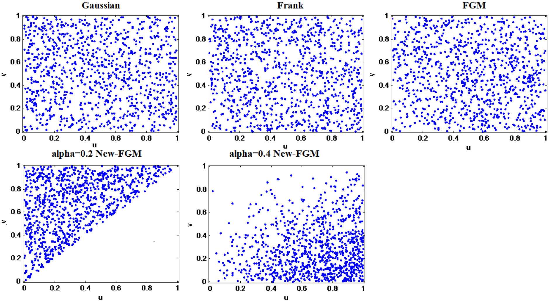
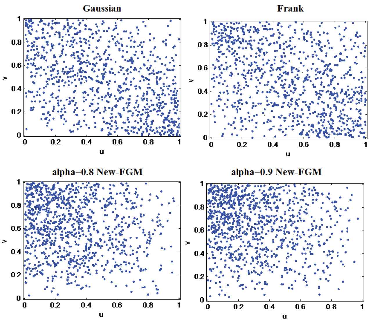
The scatter plots of the (u,v) pairs generated from the copulas for five different Kendall’s τ values is given in Figures 1–5 for different alpha possibilities, respectively. It should be attended that the Kendall τ value of the FGM copula is between [−2 / 9, 2 / 9] values. Since Kendall’s τ=−0.2561 and τ=−0.3087 values are outside these boundaries, FGM copula is not shown in Figures 4 and 5.
Figure 1
Scatter plots of the pairs (u,v) generated from copulas for τ=−0.0476.
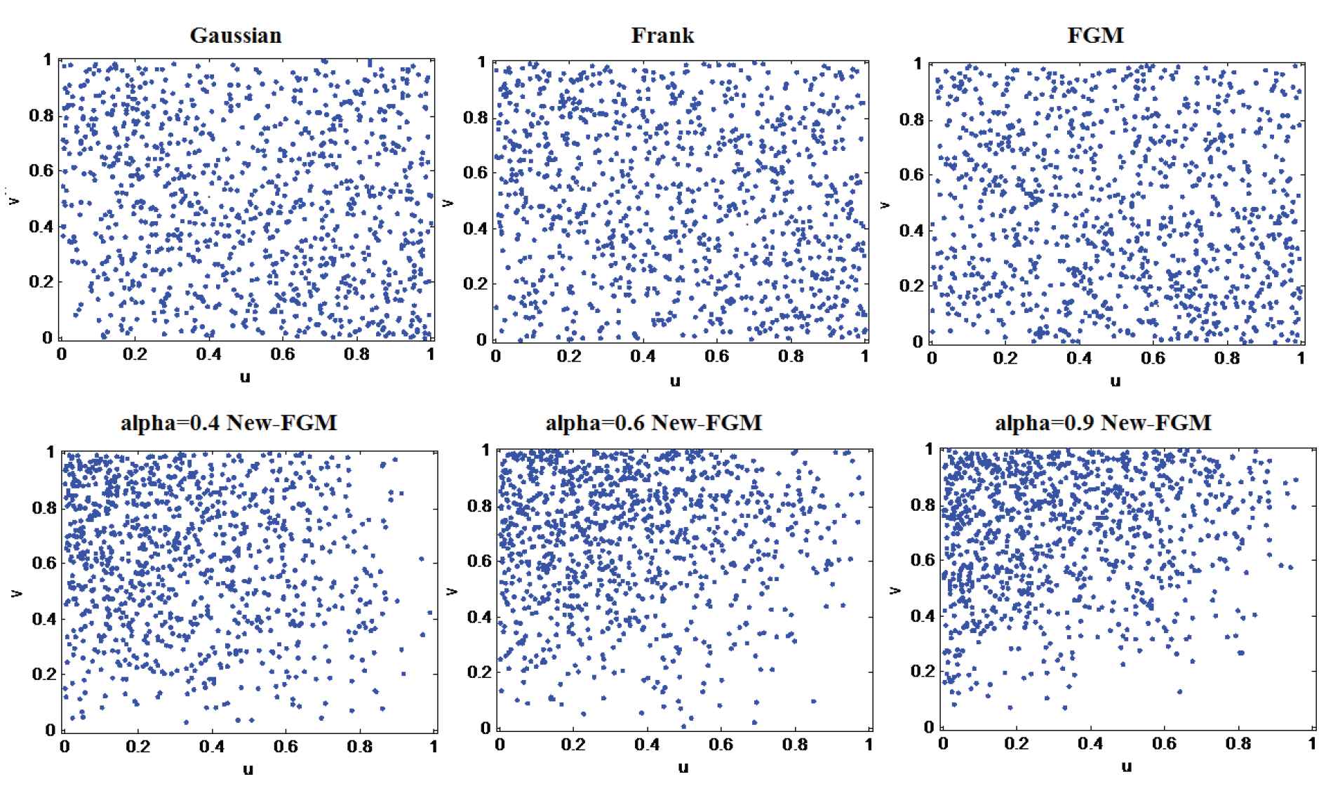
Figure 2
Scatter plots of the pairs (u,v) generated from copulas for τ=−0.1144.
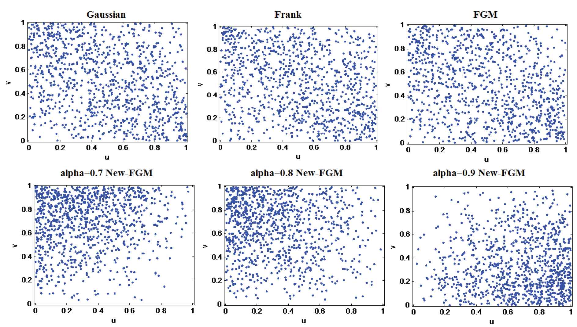
Figure 3
Scatter plots of the pairs (u,v) generated from copulas for τ=−0.2100.
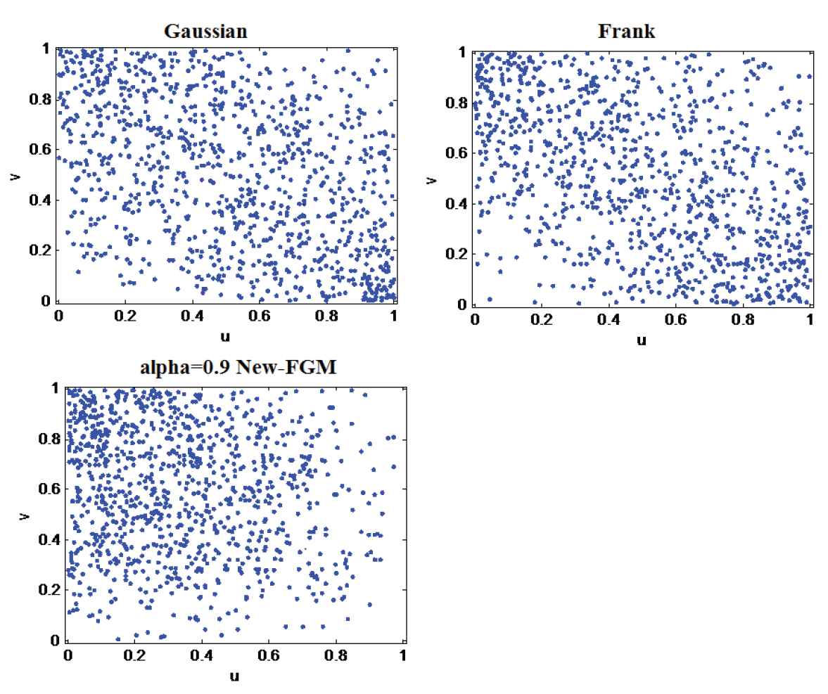
Figure 4
Scatter plots of the pairs (u,v) generated from copulas for τ=−0.2561.
Figure 5
Scatter plots of the pairs (u,v) generated from copulas for τ=−0.3087.
When the scatter plots are analyzed, it is seen that the pairs (u,v) obtained for the new form of the FGM copula reflects the negative dependency better than the other copulas. Especially, the new form of the FGM copula shows strong dependency for the small values of Kendall’s τ as absolute value.
5. CONCLUSION AND SUGGESTIONS
In this study, a new mixture copula has been obtained by means of copula proposed by Dolati and Úbeda-Flores [6]. Properties of the new mixture copula are investigated. The new mixture copula proved to be negative quadrant dependent is applied to the FGM copula. Kendall’s τ and Spearman’s ρ have been calculated for the new form of FGM copula. In addition, the new form of the FGM copula is compared with copulas appropriate to negative correlation with different alpha possibilities, without exceeding the parameter bounds. Finally, scatter plots have been obtained with creating random variables from the Gaussian, Frank and new FGM copula. When the graphics are examined, it is seen that the pairs (u,v) created from the new FGM copula reflect negative dependency, especially that it shows strong dependency for the small values of Kendall’s τ as absolute value.
It is seen, when there is a negative correlation between the variables for the new form of the FGM copula, that it gives better results than the other copulas at small correlations as absolute value. In addition, the new form of FGM mostly gives better results than the FGM copula. Also it is seen that the new FGM copula gives better results in small alpha possibilities when the negative correlations increase as absolute value. Since the new mixture copula is negative quadrant dependent, it enhances the correlation in negative side when applied to the FGM copula. Thus the new form of FGM copula can be used for higher correlations as absolute value compared to the FGM copula. Therefore, the new form of FGM copula is advised to be used when there is negative dependency between the variables.
CONFLICTS OF INTEREST
There is no conflict of interest in this article.
AUTHORS' CONTRIBUTIONS
Authors wrote the initial draft of the paper and did the analysis. Then, both of them helped in analyzing the finding and supervised overall work.
Funding Statement
We have solely funded the research by ourself.
ACKNOWLEDGMENTS
The author would like to thank the referee for their valuable suggestions and comments which improved the earlier version of the manuscript.
TY  - JOUR
AU  - Ferhan Baş Kaman
AU  - Hülya Olmuş
PY  - 2021
DA  - 2021/04/13
TI  - A New Form of Farlie-Gumbel-Morgenstern Copula: A Comparative Simulation Study and Application
JO  - Journal of Statistical Theory and Applications
SP  - 328
EP  - 339
VL  - 20
IS  - 2
SN  - 2214-1766
UR  - https://doi.org/10.2991/jsta.d.210407.001
DO  - 10.2991/jsta.d.210407.001
ID  - Kaman2021
ER  -

 , Hülya Olmuş2