
Alpha Power Transformed Weibull-G Family of Distributions: Theory and Applications

- DOI
- 10.2991/jsta.d.210222.002How to use a DOI?
- Keywords
- Application; Exponential distribution; Family of distribution; Generating function; Lindley distribution; Maximum likelihood estimation; Weibull distribution; Alpha power transformed; Distributions; Moments; Weibull -G family
- Abstract
This paper considers three special cases: Exponential, Rayleigh and Lindley of a family of generalized distributions, called alpha power Weibull G (APW-G) family. Some essential and valuable statistical properties of the family of distributions are obtained. The proposed distributions are very flexible and can be used to model data with decreasing, increasing or bathtub-shaped hazard rates. Model parameters estimation and a simulation study is carried out to evaluate the behaviors of the parameters. We consider two worthwhile data sets to illustrate the finding of the paper.
- Copyright
- © 2021 The Authors. Published by Atlantis Press B.V.
- Open Access
- This is an open access article distributed under the CC BY-NC 4.0 license (http://creativecommons.org/licenses/by-nc/4.0/).
1. INTRODUCTION
There are many classical distributions that have been developed and discussed their statistical properties and applications for various discipline in past several years. However, most of them are not suitable to model the heavy-tailed data sets (Ahmad et al. [1]). As a results, for application purposes, it is required to have the extended forms of these distributions for various fields. So, it becomes great interest among researchers to generate new univariate distributions, by adding more shape parameters to a standard distribution. The generated new distributions are more flexible in modelling data in practice. Some famous generators families are, Exponentiated -Weibull–generator (Elgarhy et al. [2]), the Marshall–Olkin - G family by Marshal and Olkin [3], beta - G family by Eugene et al. [4], the generalized odd log logistic - G by Cordeiro et al. [5], the generalized transmuted- G by Nofal et al. [6], the odd Lindley- G family by Gomes et al. [7], a new extended alpha power transformed (APT)- G by Ahmad et al. [8], a new APT- G by Elbatal et al. [9], a new power Topp-Leone- G by Bantan et al. [10], type II general inverse exponential- G by Jamal et al. [11], Truncated Inverted Kumaraswamy- G by Bantan et al. [12], the exponentiated truncated inverse Weibull-G by Almarashi et al. [13], truncated Cauchy power- G by Aldahlan et al. [14] and type II power Topp-Leone- G by Bantan et al. [15], among others.
For an arbitrary baseline cumulative distribution function (cdf)
Several properties of the
Proposed the Weibull-
The Weibull distribution is a well-known lifetime distribution and it has extensive applications in reliability theory, specifically, it is has been used for analyzing biological, medical, quality control and engineering data sets. However, when the hazard rates are bathtub, upside down bathtub or bimodal shapes, it does not work that well. As a result, in recent years, researchers are motivated to develop numerous generalizations and extensions of the Weibull distribution to model different kind of data. Therefore, the objective of this paper is to introduce a new extended generator called alpha power transformed Weibull-G (
The organization of this paper as follows. We provide the new family called
2. PROPOSED FAMILY OF DISTRIBUTIONS
Here, will construct the new generator of
The pdf of Equation (1) is given by
The survival function
2.1. Some Special of the APTW–G Models
We consider three different cases of the
| Model | |||
| Exponential | |||
| Rayleigh | |||
| Lindley |
List of few special members of the alpha power Weibull-G (APTW-G) family distribution.
Alpha power transformed Weibull exponential (
The corresponding pdf is obtained as follows:
Alpha power transformed Weibull Rayleigh (
The corresponding pdf is given by
Alpha-power transformed Weibull Lindley (APTWL) distribution
The corresponding pdf is obtained as follows:
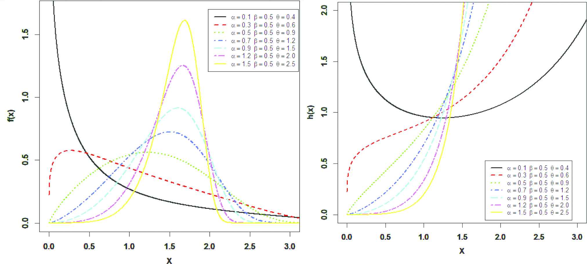
The pdf (left panel) and hazard rate function (right panel) for different set of parameters, of APTWE, APTWR and APTWL are presented in Figures 1–3 respectively.

Plots of the pdf and hrf for different parameters of the alpha power transformed Weibull exponential (APTWE) distribution.
Plots of the pdf and hrf for different parameters of the alpha power transformed Weibull Rayleigh (APTWR) distribution.
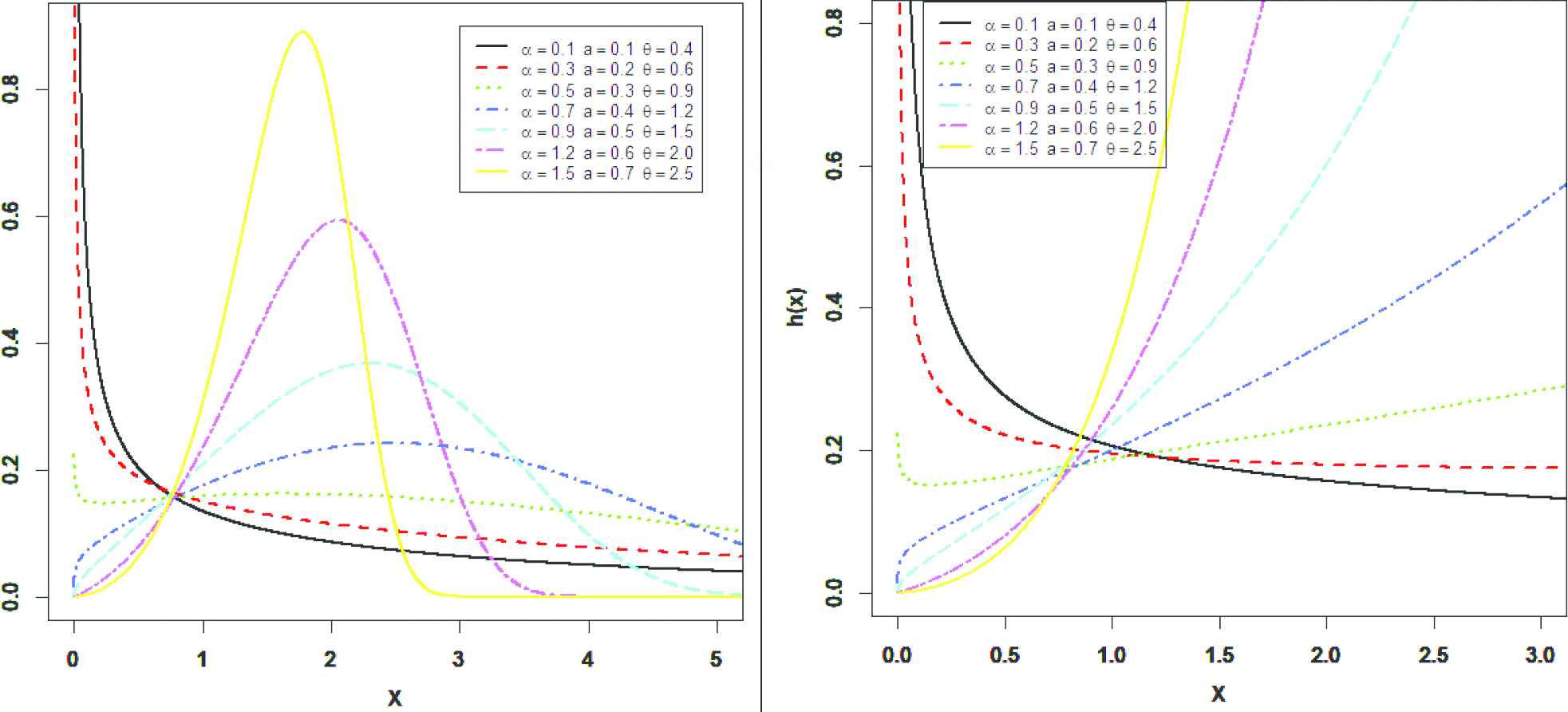
Plots of the pdf and hrf for different parameters of the alpha power transformed Weibull Lindley (APTWL) distribution.
From Figures 1–3, we observed that the pdf of APTWE, APTWR and APTWL distributions can be decreasing, symmetry, unimodal and skewed to the right, depend on the values of the parameters. Also, the hazard rate function (HRF) of APTWE, APTWR and APTWL distributions can be increasing, j- shaped, U- shaped and decreasing depend on the values of the parameters.
2.2. Expansion of the pdf of APTW–G Family
We will derive the density expansion of APTW-G family of distributions in this section. Using the power series expansion
Using the power series of the exponential function, we obtain
Furthermore, using the general binomial expansion
3. SOME STATISTICAL PROPERTIES
Most of the formulae or mathematical expressions of this paper can easily be derived using Mathematica and Maple because of their ability to deal with complex expressions.
3.1. Quantile Function
The
One can generates
3.2. Moments
The
3.3. Moment Generating Function
We display two different expressions for the moment generating function. The first one can be calculated using (9) as follows:
3.4. Conditional Moments
Here, we will discuss about the conditional moments, which are important for prediction in lifetime models. The
3.5. Mean Deviations, Bonferroni and Lorenz Curves
The mean deviations about the mean
4. MAXIMUM LIKELIHOOD ESTIMATION
Let
Using R-language, the log-likelihood can be by solving the nonlinear likelihood equations obtained by differentiating (16). The associated components of the score function
To evaluate the performance of the Maximum Likelihood (ML) of APTWE, a Monte Carlo simulation is consider. The process is arranged as follows:
We generate random samples from APTWE model.
The number of Monte Carlo replications was made 1000 times each with sample sizes 30, 50 and 100.
Selected values for the parameters are choice as reported in Tables 2–4.
Formulas used for calculating mean square error (MSE), lower bound (LB), average length (AL) and upper bound (UB) of 90% and 95% are calculated.
Step (iii) is also repeated for the other parameters.
All calculations in this section getting by using via Mathematica 9.
The simulation results for different sample sizes (30, 50 and 100) and different values of parameters
| 90% |
95% |
|||||||
|---|---|---|---|---|---|---|---|---|
| n | MLE | MSE | LB | UB | AL | LB | UB | AL |
| 30 | 0.591 | 0.031 | 0.194 | 0.989 | 0.795 | 0.118 | 1.065 | 0.947 |
| 0.627 | 0.222 | −0.361 | 1.615 | 1.977 | −0.551 | 1.805 | 2.355 | |
| 0.614 | 0.073 | 0.219 | 1.008 | 0.79 | 0.143 | 1.084 | 0.941 | |
| 50 | 0.476 | 0.007 | 0.293 | 0.659 | 0.366 | 0.258 | 0.694 | 0.436 |
| 0.434 | 0.057 | −0.002 | 0.871 | 0.873 | −0.086 | 0.954 | 1.04 | |
| 0.541 | 0.009 | 0.389 | 0.693 | 0.304 | 0.36 | 0.723 | 0.362 | |
| 100 | 0.506 | 0.004 | 0.385 | 0.628 | 0.242 | 0.362 | 0.651 | 0.289 |
| 0.572 | 0.043 | 0.232 | 0.911 | 0.679 | 0.167 | 0.976 | 0.809 | |
| 0.488 | 0.003 | 0.412 | 0.564 | 0.151 | 0.398 | 0.578 | 0.18 | |
Numerical results for APTWE model at (
| 90% |
95% |
|||||||
|---|---|---|---|---|---|---|---|---|
| n | MLE | MSE | LB | UB | AL | LB | UB | AL |
| 30 | 1.2770 | 1.3630 | −0.1010 | 2.6550 | 2.7570 | −0.3650 | 2.9190 | 3.2850 |
| 0.9560 | 1.1530 | −0.5940 | 2.5070 | 3.1010 | −0.8910 | 2.8040 | 3.6950 | |
| 0.4950 | 0.0050 | 0.3760 | 0.6150 | 0.2390 | 0.3530 | 0.6380 | 0.2850 | |
| 50 | 0.8890 | 0.0770 | 0.5180 | 1.2610 | 0.7420 | 0.4470 | 1.3320 | 0.8850 |
| 0.6290 | 0.1920 | 0.1060 | 1.1530 | 1.0470 | 0.0060 | 1.2530 | 1.2470 | |
| 0.5140 | 0.0040 | 0.4200 | 0.6090 | 0.1890 | 0.4010 | 0.6270 | 0.2250 | |
| 100 | 0.7950 | 0.0060 | 0.5680 | 1.0230 | 0.4550 | 0.5240 | 1.0660 | 0.5420 |
| 0.4970 | 0.0130 | 0.2070 | 0.7880 | 0.5810 | 0.1510 | 0.8440 | 0.6920 | |
| 0.5020 | 0.0010 | 0.4300 | 0.5740 | 0.1430 | 0.4170 | 0.5870 | 0.1710 | |
Numerical results for APTWE model at (
| 90% |
95% |
|||||||
|---|---|---|---|---|---|---|---|---|
| n | MLE | MSE | LB | UB | AL | LB | UB | AL |
| 30 | 0.929 | 0.115 | 0.365 | 1.492 | 1.128 | 0.257 | 1.6 | 1.343 |
| 1.012 | 0.298 | −0.157 | 2.181 | 2.338 | −0.381 | 2.405 | 2.786 | |
| 0.493 | 0.004 | 0.367 | 0.619 | 0.251 | 0.343 | 0.643 | 0.3 | |
| 50 | 0.894 | 0.057 | 0.539 | 1.249 | 0.71 | 0.471 | 1.317 | 0.846 |
| 0.933 | 0.135 | 0.243 | 1.823 | 1.58 | 0.092 | 1.974 | 1.882 | |
| 0.486 | 0.002 | 0.402 | 0.571 | 0.17 | 0.385 | 0.588 | 0.202 | |
| 100 | 0.849 | 0.026 | 0.603 | 1.096 | 0.493 | 0.555 | 1.143 | 0.588 |
| 0.759 | 0.085 | 0.321 | 1.197 | 0.877 | 0.237 | 1.281 | 1.044 | |
| 0.509 | 0.001 | 0.452 | 0.605 | 0.153 | 0.438 | 0.619 | 0.182 | |
Numerical results for APTWE model at (
5. APPLICATIONS
For illustration purposes of the APTWE model, two real data sets are analyzed in this section. The first data was consider by Linhart and Zucchini [22], which signifies the failure times of air-conditioned system of an airplane. The second data set was consider by Aarset [23], which represents the failure times of 50 devices. All data sets are presented in Table 5. We fit the APTWE distribution and other four competing models namely; alpha power transformed Weibull inverse Lomax (APTIL) (ZeinEldein et al. [24]), alpha power transformed Lindley (APTL) (Dey et al. [17]), alpha power transformed exponential (APTE) (Mahadavi and Kundu [16]) distributions. The probability densities of these distributions is given by:
| Data 1 | 23, 261, 87, 7, 120, 14, 62, 47, 225, 71, 246, 21, 42, 20, 5, 12, 120, 11, 3, 14, 71, 11, 14, 11, 16, 90, 1, 16, 52, 95 |
| Data 2 | 0.1, 0.2, 1, 1, 1, 1, 1, 2, 3, 6, 7, 11, 12, 18, 18, 18, 18, 18, 21, 32, 36, 40, 45, 46, 47, 50, 55, 60, 63, 63, 67, 67, 67, 67, 72, 75, 79, 82, 82, 83, 84, 84, 84, 85, 85, 85, 85, 85, 86, 86 |
Failures time data.
Figures 4 and 5 demonstrate the box and TTT plots for the two datasets respectively. Aarset (1987) proposed that the hrf is decreasing or increasing if the graph of TTT plot is a convex or concave. The hrf is U-shaped (bathtub) if the TTT plot is firstly convex and then concave.
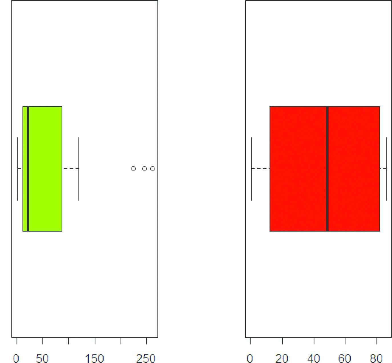
Box plots of both data sets.
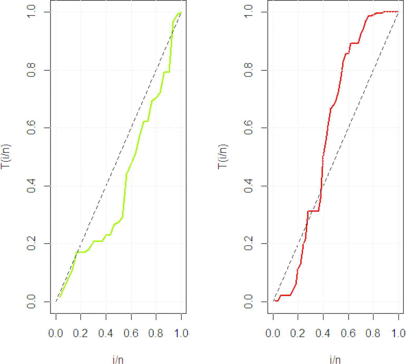
TTT plots of both data sets.
The ML estimates along with their standard error (SE) of the model parameters for the first and second sets are provided in Tables 6 and 7 respectively. In the same tables, the analytical measures including; minus log-likelihood (-log L) Kolmogorov–Smirnov (KS) test statistic, Akaike information criterion (AIC), corrected Akaike information criterion (CAIC), Bayesian information criterion (BIC) and Hannan–Quinn information criterion (HQIC) are presented.
| Model | ML Estimates (SE) | −Log L | AIC | BIC | CAIC | HQIC | KS |
|---|---|---|---|---|---|---|---|
| APTWE | 176.788 | 359.576 | 358.007 | 360.499 | 360.92 | 0.1497 | |
| APTIL | 177.573 | 361.146 | 359.578 | 361.668 | 362.491 | 0.2007 | |
| APTL | 183.415 | 370.83 | 369.784 | 371.274 | 371.727 | 0.2803 | |
| APTE | 177.388 | 358.775 | 357.729 | 359.22 | 359.672 | 0.19989 |
APTWE, Alpha power transformed Weibull exponential; SE, standard error; −Log L, minus log-likelihood; APTIL, alpha power transformed Weibull inverse Lomax; APTL, alpha power transformed Lindley; APTE. alpha power transformed exponential; AIC, Akaike information Criterion; BIC, Bayesian information criterion; CAIC, corrected Akaike information criterion; HQIC, Hannan–Quinn information criterion; KS, Kolmogorov–Smirnov test statistic
Analytical results of the APTWE model and other competing models for the first data set.
| Model | ML Estimates (SE) | −Log L | AIC | BIC | CAIC | HQIC | KS |
|---|---|---|---|---|---|---|---|
| APTWE | 269.911 | 545.823 | 544.92 | 546.344 | 548.007 | 0.14042 | |
| APTIL | 291.608 | 589.217 | 588.314 | 589.739 | 591.401 | 0.2677 | |
| APTL | 296.747 | 597.495 | 596.892 | 597.939 | 598.951 | 0.2186 | |
| APTE | 283.583 | 571.167 | 570.565 | 571.611 | 572.623 | 0.19311 |
APTWE, Alpha power transformed Weibull exponential; SE, standard error; −Log L, minus log-likelihood; APTIL, alpha power transformed Weibull inverse Lomax; APTL, alpha power transformed Lindley; APTE. alpha power transformed exponential; AIC, Akaike information Criterion; BIC, Bayesian information criterion; CAIC, corrected Akaike information criterion; HQIC, Hannan–Quinn information criterion; KS, Kolmogorov–Smirnov test statistic
Analytical results of the APTWE model and other competing models for the second data set.
From Tables 6 and 7, it is evident that the proposed APWE distribution provides the overall best fit and therefore could be chosen as the more adequate model among APTWE, APTIL, APTL and APTE models. We also plotted epdf, ecdf, esf and PP plots in Figures 6 and 7 for first and second data sets respectively.
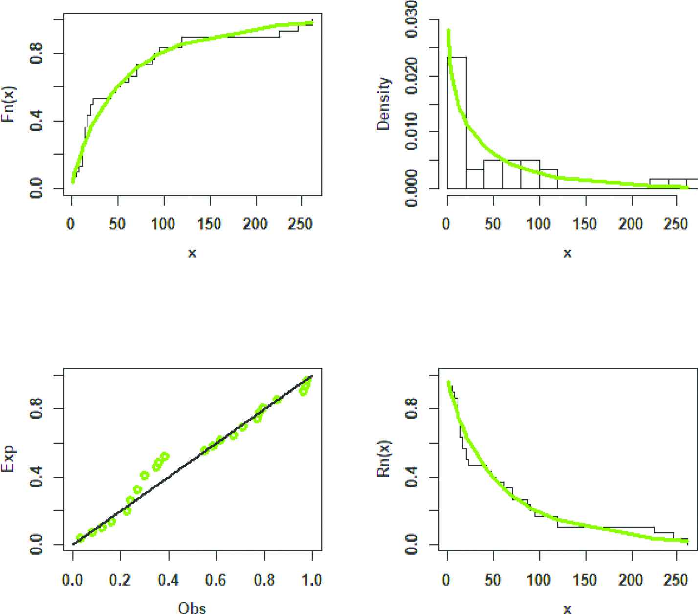
ecdf, epdf, PP plots and esf for the first dataset.
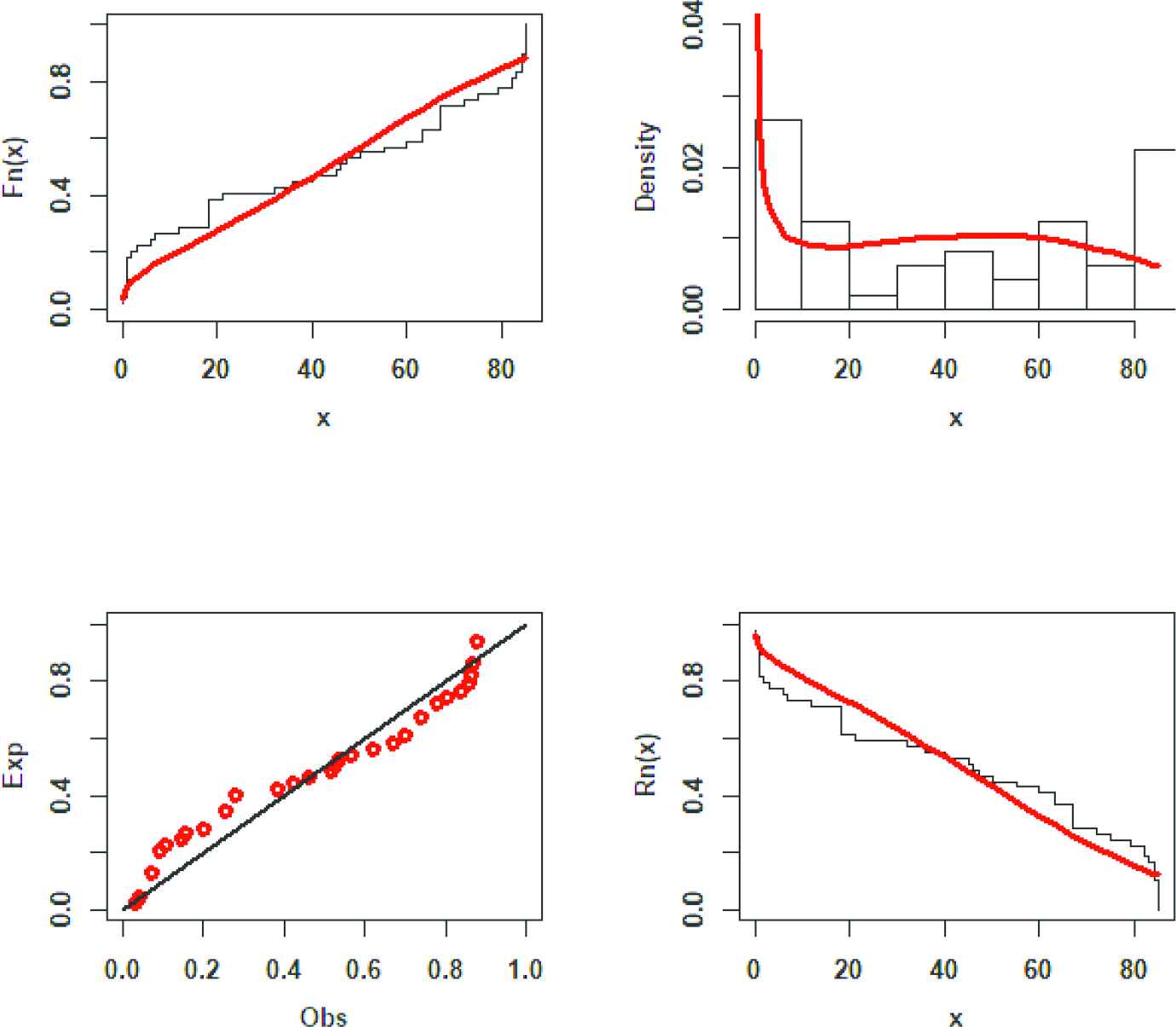
ecdf, epdf, PP plots and esf for the second dataset.
6. CONCLUSIONS
In this paper, we developed three special cases (Exponential, Rayleigh and Lindley) of the family of generalized distributions, called APW-G family. The density function of the proposed models can have numerous forms: increasing, decreasing, negatively-skewed, positively skewed or symmetrical depend on the values of parameters. Some of useful statistical properties, such as expansion of density function, moments, generating function, incomplete moments, mean deviation, Bonferroni and Lorenz curves are provided. We also discuss the method of maximum likelihood to estimate the model parameters. The performance of the new family of distributions is illustrated by means of a four real data sets. It is observed that the proposed distribution perform well than some competitive distributions. It is expected that this paper will be useful for the users or researchers, those are listed in Section 1.
CONFLICTS OF INTEREST
The authors declar no conflict of interest.
AUTHORS' CONTRIBUTIONS
All authors have equally contributed for the manuscript.
ACKNOWLEDGMENTS
Authors are grateful to anonymous referees for their valuable comments and suggestions, which improved the quality and presentation of the paper greatly. Author, B. M. Golam Kibria wants to dedicate this paper to his very favorite teacher, Late Prof. M Kabir, Department of Statistics, Jahangirnagar University, Bangladesh for his wisdom, constant inspiration during student life and affection that motivated him to achieve this present position.
APPENDIX
REFERENCES
Cite this article
TY  - JOUR
AU  - I. Elbatal
AU  - M. Elgarhy
AU  - B. M. Golam Kibria
PY  - 2021
DA  - 2021/03/01
TI  - Alpha Power Transformed Weibull-G Family of Distributions: Theory and Applications
JO  - Journal of Statistical Theory and Applications
SP  - 340
EP  - 354
VL  - 20
IS  - 2
SN  - 2214-1766
UR  - https://doi.org/10.2991/jsta.d.210222.002
DO  - 10.2991/jsta.d.210222.002
ID  - Elbatal2021
ER  -