
Optimum Ridge Regression Parameter Using R-Squared of Prediction as a Criterion for Regression Analysis
- DOI
- 10.2991/jsta.d.210322.001How to use a DOI?
- Keywords
- Ridge parameter; PRESS; Maximization of R2-prediction; Model prediction power
- Abstract
The presence of the multicollinearity problem in the predictor data causes the variance of the ordinary linear regression coefficients to be increased so that the prediction power of the model not to be satisfied and sometimes unacceptable results be predicted. The ridge regression has been proposed as an efficient method to combat multicollinearity problem long ago. In application of ridge regression the researcher uses the ridge trace and selects a value of ridge parameter in such a manner that he thinks the regression coefficients have stabilized; this leads the ridge regression to be subjective technique. The purpose of this paper is the conversion of the ridge regression method from a qualitative method to a quantitative one meanwhile to present a method to find the optimum ridge regression parameter which maximizes the R-squared of prediction. We examined four well-known case studies on this regard. Significant improvements at all of the cases demonstrated the validity of our proposed method.
- Copyright
- © 2021 The Authors. Published by Atlantis Press B.V.
- Open Access
- This is an open access article distributed under the CC BY-NC 4.0 license (http://creativecommons.org/licenses/by-nc/4.0/).
1. INTRODUCTION
In many scientific and engineering disciplines, the researchers face to study the effect of some input or predictor variables on an output or response variable. After performing experiments, which are usually done either in classical one-factor-at-time method or using experimental design patterns, there is a need to relate the input variables to output variable via a characterizing mathematical relationship. Hence, if there is a theoretical relationship between Y and X, then the form of the relating function will be specified. If the theoretical functionality has not been developed, then the researcher may use empirical linear models using some parameter β. The values of these parameters can be estimated by using linear regression technique [7,8,18,30,36,37,39,40,41,48].
Sometimes the number of predictor variables is large or predictors are not really independent and there may be some correlations between input variables. In these cases, the relationship Xi. Xj = 0 dose not satisfy. The presence of correlation between predictor variables produces the multicollinearity problem. The effects of collinearity have been discussed by above mentioned researchers and also by Gunst [19], Jensen and Ramirez [28].
The significant number of methods has been proposed to overcome multicollinearity problem (e.g., see [3,14,15,17,41]).
One of the efficient methods to combat the multicollinearity problems is ridge regression developed by Hoerl [23], Hoerl and Kennard [24,25] for the first time. Many researchers used it in practice and found it useful on this regard for example see Marquardt [33], Hemmerle [20], Marquardt and Snee [34], Khuri and Myers [30], Dorugade [5], Fitrianto and Yik [13], Yahya and Olaifa [48].
Hoerl and Kennard [26] themselves published the first review paper on ridge regression and then other reviews appeared in the literature, among them, the works of Singh [43], Dube and Isha [9], Duzan and Shariff [10], Goktas and Sevinc [16] can be mentioned.
Some of the researchers tried to show the application and usefulness of ridge regression using simulation studies [6,11,27,32,42].
On the other hand some researchers criticized the ridge regression method from different points of view for example see Smith and Campbel [44], and also the comments of Thisted et al. were appeared in the same issue of Journal of American Statistical Association (1980); Draper and Smith [7], Singh [43], Chatterjee and Hadi [3].
One of the main weaknesses of the ridge regression is that the ridge regression parameter can be selected by examining the ridge trace (Marquardt and Snee [34] points out that for using ridge regression 25 values of k in the interval of [0 1] need to be examined).
A large number of methods have been proposed to calculate the ridge parameter (see [9,10,16,33,43] compare 39 methods of estimating ridge parameters). By considering these at all; one may conclude that the ridge regression is a subjective method. The first objective of this paper is to convert the ridge regression method from a qualitative method to a quantitative one meanwhile the second objective is to present a method to find the optimum ridge regression parameter which maximizes the prediction power of a given model using ridge regression with optimum ridge parameter.
2. METHOD
As is obvious one of the main reasons for making a good model from data is not merely the prediction of the given responses from predictor variables, and we are also interested in predicting the values of response at other conditions where there are not any data. Hence the prediction power of the model is so crucial. The R-squared of prediction and also prediction residual sum of squares can be considered as good measures on this regard [1,2,4,12,17,22]. Let us below have a look on the related formula:
This can be obtained using leave-one-out cross-validation technique. The PRESS residual for ith data is
The values of hii are the diagonal elements of the hat matrix associated with ridge regression parameter calculated below.
In this equation X is predictors matrix with 1's in the first column, X’ is the transpose of the predictors matrix, I is the identity matrix, k is the ridge regression parameter, and β* is the coefficients of the given model using ridge regression technique. If k equals zero the ridge regression converts to the ordinary least square regression.
We propose that the value of ridge regression parameter which maximizes the R2-prediction is said to be the optimum ridge parameter, the numerical value of the ridge parameter k, can be obtained by using an optimizer via trial and error operation.
3. RESULTS AND DISCUSSION
In order to illustrate the validity of our method to determine the optimum ridge regression parameter we will deal with four examples namely acetylene conversion, French import economy, heat evolved on cement hardening, and propellant mechanical property.
3.1. Acetylene Conversion
Original data of converting normal heptane to acetylene were collected by Kunugi et al. [31]. Himmelblau [21], presented information of this conversion data which were used by other researchers as a classical example when they dealt with ridge regression to overcome the multicollinearity problem (see [34,35,37,45,46]).
Here we will consider four different models to show the application of our proposed method, namely main effect model, interaction model, reduced model, and full quadratic model as below:
Here, as mentioned by Marquardt and Snee [34]; X1*, X2*, and X3* are the centered and scaled forms of the original variables as defined below:
The coefficients of ai’s, bi’s, ci’s, and di’s could easily be calculated using ordinary least squares technique.
Table 1 presents the X matrix for main effect model, whereas in Table 2 the statistics of PRESS, R2, SST, and also R2-prediction at different values of ridge parameter for main effect model are tabulated.
| X1* | X2* | X3* | |
|---|---|---|---|
| 1 | 1.085304 | −0.87314 | −0.89487 |
| 1 | 1.085304 | −0.60822 | −0.89487 |
| 1 | 1.085304 | −0.25499 | −0.91068 |
| 1 | 1.085304 | 0.18655 | −0.86327 |
| 1 | 1.085304 | 0.804702 | −0.84746 |
| 1 | 1.085304 | 1.864392 | −0.89487 |
| 1 | −0.15504 | −1.26169 | −0.00988 |
| 1 | −0.15504 | −0.87314 | −0.07309 |
| 1 | −0.15504 | −0.25499 | −0.26273 |
| 1 | −0.15504 | 0.18655 | −0.45238 |
| 1 | −0.15504 | 0.804702 | −0.19952 |
| 1 | −0.15504 | 1.864392 | 0.02173 |
| 1 | −1.39539 | −1.26169 | 1.380833 |
| 1 | −1.39539 | −0.87314 | 1.823331 |
| 1 | −1.39539 | −0.25499 | 1.633689 |
| 1 | −1.39539 | 0.804702 | 1.444047 |
Predictors matrix, X for main effect model of acetylene data.
| Ridge, k | 0 | 0.04 | 0.016 | 0.064 | 0.128 | 0.178743 | 0.256 | 0.512 |
|---|---|---|---|---|---|---|---|---|
| PRESS | 336.2955 | 332.3246 | 334.5347209 | 330.5745 | 327.785 | 327.1727 | 328.4182 | 346.5632 |
| R2 | 0.919815 | 0.919768 | 0.919806742 | 0.919703 | 0.91944 | 0.919172 | 0.918715 | 0.917167 |
| SST | 2123.709 | 2123.709 | 2123.709375 | 2123.709 | 2123.709 | 2123.709 | 2123.709 | 2123.709 |
| R2-pred | 0.841647 | 0.843517 | 0.842476224 | 0.844341 | 0.845654 | 0.845943 | 0.845356 | 0.836812 |
Statistics for main effect model at different values of k parameter.
Tables 3 and 4 show those statistics for interaction and reduced models respectively.
| Ridge, k | 0 | 0.004 | 0.016 | 0.032 | 0.054155 | 0.064 | 0.128 | 0.256 |
|---|---|---|---|---|---|---|---|---|
| PRESS | 46.3023 | 44.54459 | 41.01827 | 38.77256 | 37.96507 | 38.07526 | 41.79881 | 55.08884 |
| R2 | 0.994565 | 0.994561 | 0.994518 | 0.99441 | 0.994207 | 0.994104 | 0.993332 | 0.991444 |
| SST | 2123.709 | 2123.709 | 2123.709 | 2123.709 | 2123.709 | 2123.709 | 2123.709 | 2123.709 |
| R2-pred | 0.978197 | 0.979025 | 0.980686 | 0.981743 | 0.982123 | 0.982071 | 0.980318 | 0.97406 |
Statistics for interaction model at different values of k parameter.
| Ridge, k | 0 | 0.001 | 0.004 | 0.005 | 0.006667 | 0.01 | 0.015 | 0.02 |
|---|---|---|---|---|---|---|---|---|
| PRESS | 37.82797 | 37.79893 | 37.74268 | 37.73343 | 37.72765 | 37.74905 | 37.85204 | 38.0249 |
| R2 | 0.993708 | 0.993708 | 0.993703 | 0.993701 | 0.993696 | 0.993681 | 0.993652 | 0.993613 |
| SST | 2123.709 | 2123.709 | 2123.709 | 2123.709 | 2123.709 | 2123.709 | 2123.709 | 2123.709 |
| R2-pred | 0.982188 | 0.982201 | 0.982228 | 0.982232 | 0.982235 | 0.982225 | 0.982176 | 0.982095 |
Statistics for reduced model at different values of k parameter.
The variations of those statistics for full quadratic model are demonstrated in Figures 1–3.

R-square for full quadratic model.
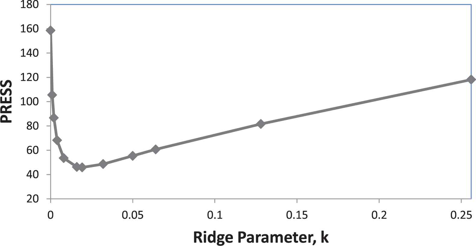
PRESS for full quadratic model.
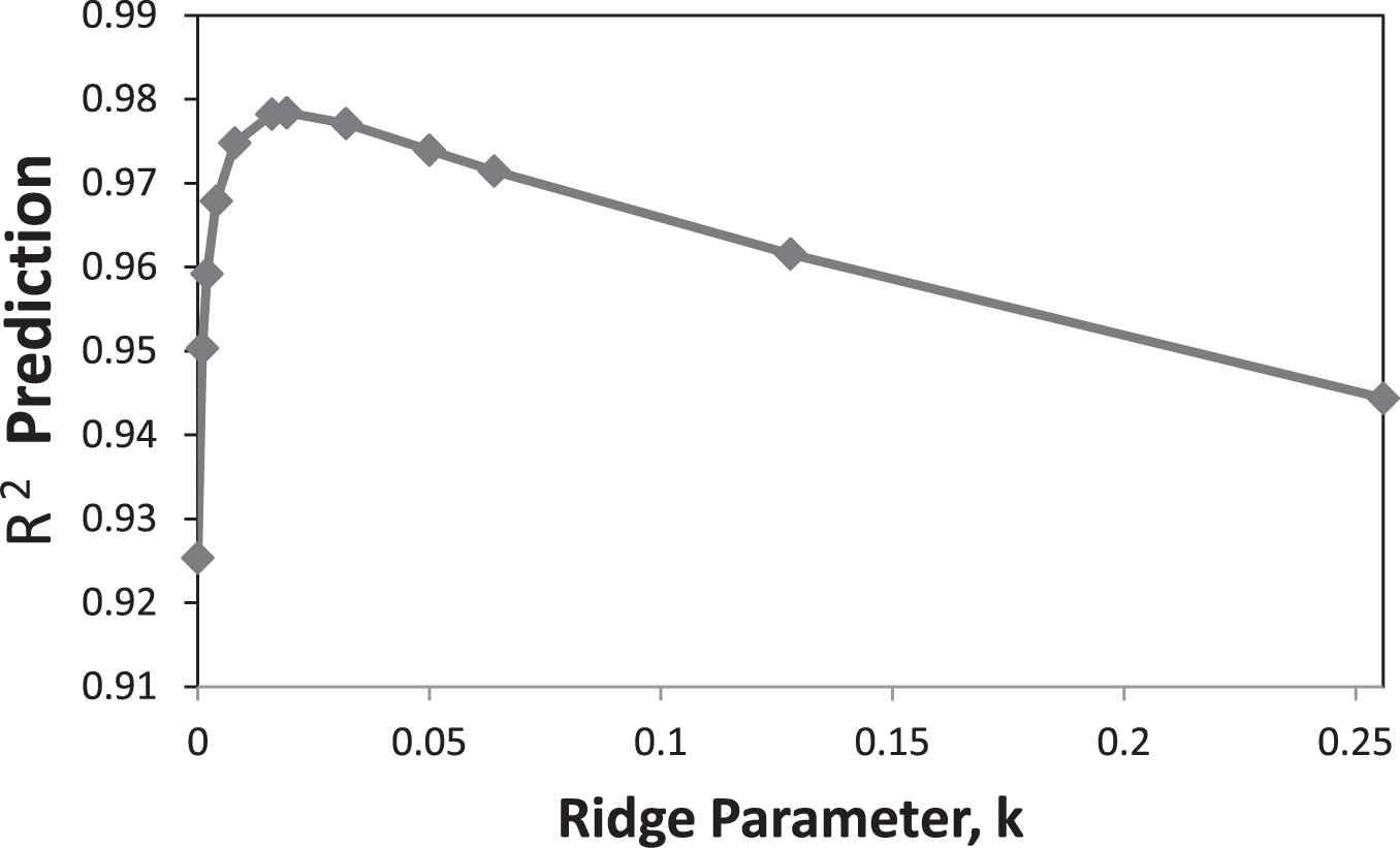
R2-prediction for full quadratic model.
The data for Figure 4 have been obtained from Myers and Montgomery ([37] Table A.2.4 page 678).
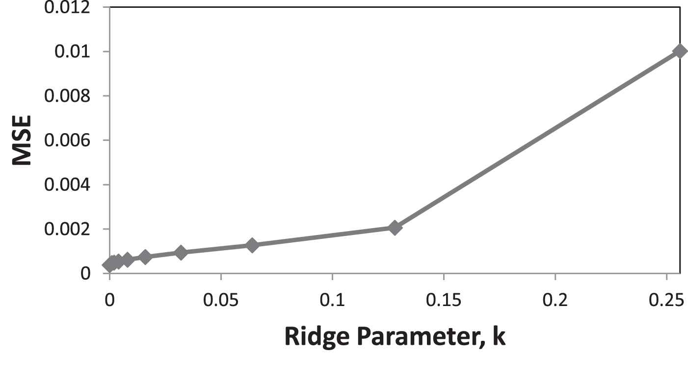
Mean squared of error for full quadratic model.
Investigation of the data reveal that there is an optimum value for ridge regression parameter k, where PRESS is at minimum and R2-prediction at the maximum value. Bold numbers show the optimum ridge parameter and its corresponding statistics in Tables 2–4.
Comparison of those statistics for full quadratic model at k = 0, with the corresponding values of ridge parameters proposed by other researchers (Maraquardt and Snee, 1975, and Snee [46], k = 0.01, 0.05; Myers and Montgomery [37], and Montgomery et al. [35], k = 0.008, 0.032, and 0.064), and also at optimum value of ridge regression parameter are illustrated in Table 5.
| OLS | Opt-RR | ||||||
|---|---|---|---|---|---|---|---|
| Ridge, k | 0.00000 | 0.00800 | 0.01000 | 0.01923 | 0.03200 | 0.05000 | 0.06400 |
| PRESS | 158.56920 | 53.54655 | 50.23883 | 45.89658 | 48.63185 | 55.36370 | 60.67380 |
| R2 | 0.99770 | 0.99719 | 0.99712 | 0.99677 | 0.99622 | 0.99540 | 0.99476 |
| SST | 2123.70938 | 2123.70938 | 2123.70938 | 2123.70938 | 2123.70938 | 2123.70938 | 2123.70938 |
| R2-PRED | 0.92533 | 0.97479 | 0.97634 | 0.97839 | 0.97710 | 0.97393 | 0.97143 |
Comparison of statistics at different values of ridge parameter for full quadratic model which have been proposed by other researchers.
Examination of the data in Table 5 shows that there are two important points. The first one is existing improvements in the values of PRESS and R2-prediction at all proposed values of ridge parameters against ordinary least square. The next issue is that the most significant improvement in PRESS and R2-prediction appear at the optimum value of the ridge regression parameter where PRESS is at lowest and R2-rediction is at highest value. Comparison of the PRESS and R2-prediction for different models at their optimum ridge parameter, show that our method can also be used as a criterion for model selection too, on this regard the models using optimum k can be arranged in the following merit order:
3.2. French Economy
The French Import data for the years 1949–1966 were presented and analyzed by Chatterjee and Hadi [3], using principal component as well as ridge regression analysis. The three predictor variables were domestic production, stock formation, and domestic consumption; the response variable is French import; predictor and response variables are all in billions of francs.
They reported three values for ridge regression parameter using Hoerl et al. [27] equation (0.0164); Hoerl and Kennard [25] iterative method (0.0161); and investigating the ridge trace (0.04) where it is stabilized.
Figure 5 shows the variation of PRESS as a function of ridge parameter, whereas Figure 6 demonstrates the variation of R2-prediction versus k.
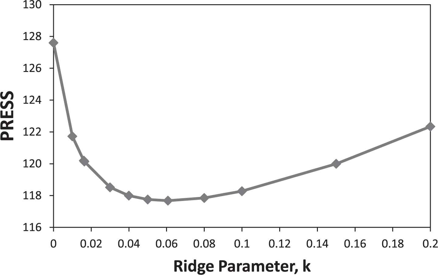
PRESS for French import economy data.
R2-prediction for French import economy data.
The optimum value for ridge parameter in this example was calculated as 0.06074 where the crest and hill for PRESS and R2-prediction appears as shown in related figures.
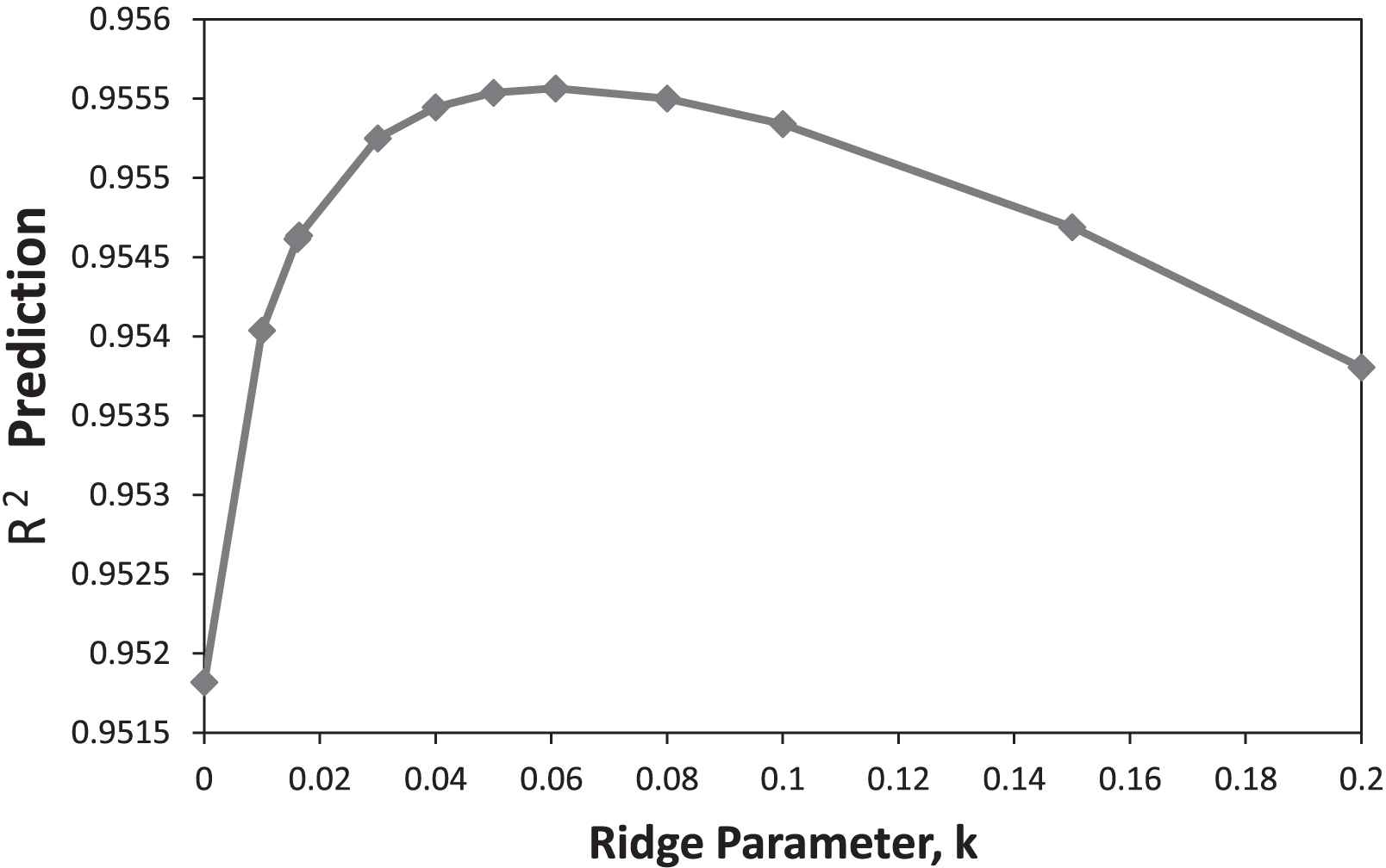
3.3. Hald Data for Portland Cement Composition
The data set for Hald data can be found in Appendices B and C of Draper and Smith [7], and also in Table 10.10 of Chatterjee and Hadi [3]. The aim of the study was to investigate the amount of heat evolved during the cement hardening as a function of Portland cement constituents. Centered and scaled of the Hald data provides the predictor matrix of X, tabulated in Table 6.
| X1* | X2* | X3* | X4* | |
|---|---|---|---|---|
| 1 | −0.07846 | −1.42369 | −0.90072 | 1.79231 |
| 1 | −1.09845 | −1.2309 | 0.504404 | 1.31436 |
| 1 | 0.601534 | 0.504223 | −0.58847 | −0.59744 |
| 1 | 0.601534 | −1.10237 | −0.58847 | 1.015642 |
| 1 | −0.07846 | 0.247168 | −0.90072 | 0.179231 |
| 1 | 0.601534 | 0.439959 | −0.43235 | −0.47795 |
| 1 | −0.75846 | 1.468179 | 0.816654 | −1.43385 |
| 1 | −1.09845 | −1.10237 | 1.597278 | 0.836411 |
| 1 | −0.92845 | 0.375696 | 0.972779 | −0.47795 |
| 1 | 2.301522 | −0.07415 | −1.21297 | −0.23897 |
| 1 | −1.09845 | −0.524 | 1.753403 | 0.238975 |
| 1 | 0.601534 | 1.14686 | −0.43235 | −1.07539 |
| 1 | 0.431535 | 1.275388 | −0.58847 | −1.07539 |
Predictors matrix, X for main effect model of Hald data.
Draper and Smith (1987) reported a value for ridge regression parameter using Hoerl et al. [27] equation (0.0131). In Table 7 we report the statistics of PRESS, R2, SST, and also R2-prediction at different values of ridge parameter for the main effect model. We observe the crest for PRESS and hill for R2-prediction appear at ridge parameter of 0.02991, which is the optimum value.
| OLS | Opt-RR | |||||||
|---|---|---|---|---|---|---|---|---|
| Ridge, k | 0 | 0.01 | 0.0131 | 0.02 | 0.02991 | 0.05 | 0.08 | 0.1 |
| PRESS | 110.3466 | 100.6498 | 99.45204 | 97.92197 | 97.29514 | 98.99015 | 105.8798 | 112.6457 |
| R2 | 0.982376 | 0.982347 | 0.982336 | 0.982312 | 0.982284 | 0.982243 | 0.982201 | 0.982179 |
| SST | 2715.763 | 2715.763 | 2715.763 | 2715.763 | 2715.763 | 2715.763 | 2715.763 | 2715.763 |
| R2-Pred | 0.959368 | 0.962939 | 0.96338 | 0.963943 | 0.964174 | 0.96355 | 0.961013 | 0.958522 |
Comparison statistics at different values of ridge parameter for main effect model.
3.4. Propellant Property
The data set for mechanical property of propellant data were presented by Khuri and Myers [30], and also in Table 5.12 of Khuri and Cornell [29]. The aim of the study was to maximize the certain mechanical modular property of propellant as a function concentration of three substances. Due to practical problems, instead of central composite design they used deformed Central Composite Design (CCD) design for doing experiments which caused multicollinearity problem.
Since they reported the coded data, without centering and scaling, the predictor matrix is tabulated in Table 8. For this example we report the statistics of Total prediction residual sum of squares (PRESS), R2, SST, and also R2-prediction at different values of ridge parameter in Table 9.
| X1 | X2 | X3 | X1X2 | X1X3 | X2X3 | X1X1 | X2X2 | X3X3 | |
|---|---|---|---|---|---|---|---|---|---|
| 1 | −1.0200 | −1.4020 | −0.9980 | 1.4300 | 1.0180 | 1.3992 | 1.0404 | 1.9656 | 0.9960 |
| 1 | 0.9000 | 0.4780 | −0.8180 | 0.4302 | −0.7362 | −0.3910 | 0.8100 | 0.2285 | 0.6691 |
| 1 | 0.8700 | −1.2820 | 0.8820 | −1.1153 | 0.7673 | −1.1307 | 0.7569 | 1.6435 | 0.7779 |
| 1 | −0.9500 | 0.4580 | 0.9720 | −0.4351 | −0.9234 | 0.4452 | 0.9025 | 0.2098 | 0.9448 |
| 1 | −0.9300 | −1.2420 | −0.8680 | 1.1551 | 0.8072 | 1.0781 | 0.8649 | 1.5426 | 0.7534 |
| 1 | 0.7500 | 0.4980 | −0.6180 | 0.3735 | −0.4635 | −0.3078 | 0.5625 | 0.2480 | 0.3819 |
| 1 | 0.8300 | −1.0920 | 0.7320 | −0.9064 | 0.6076 | −0.7993 | 0.6889 | 1.1925 | 0.5358 |
| 1 | −0.9500 | 0.3780 | 0.8320 | −0.3591 | −0.7904 | 0.3145 | 0.9025 | 0.1429 | 0.6922 |
| 1 | 1.9500 | −0.4620 | 0.0020 | −0.9009 | 0.0039 | −0.0009 | 3.8025 | 0.2134 | 0.0000 |
| 1 | −2.1500 | −0.4020 | −0.0380 | 0.8643 | 0.0817 | 0.0153 | 4.6225 | 0.1616 | 0.0014 |
| 1 | −0.5500 | 0.0580 | −0.5180 | −0.0319 | 0.2849 | −0.0300 | 0.3025 | 0.0034 | 0.2683 |
| 1 | −0.4500 | 1.3780 | 0.1820 | −0.6201 | −0.0819 | 0.2508 | 0.2025 | 1.8989 | 0.0331 |
| 1 | 0.1500 | 1.2080 | 0.0820 | 0.1812 | 0.0123 | 0.0991 | 0.0225 | 1.4593 | 0.0067 |
| 1 | 0.1000 | 1.7680 | −0.0080 | 0.1768 | −0.0008 | −0.0141 | 0.0100 | 3.1258 | 0.0001 |
| 1 | 1.4500 | −0.3420 | 0.1820 | −0.4959 | 0.2639 | −0.0622 | 2.1025 | 0.1170 | 0.0331 |
Predictors matrix, X for quadratic model of propellant data.
| OLS | Opt-RR | |||||||
|---|---|---|---|---|---|---|---|---|
| Ridge, k | 0 | 0.01 | 0.05 | 0.11055 | 0.2 | 0.4 | 0.6 | 0.8 |
| PRESS | 425.924458 | 309.6907 | 132.8877 | 96.01921 | 113.2438 | 156.5302 | 181.3001 | 196.5669 |
| R2 | 0.97380208 | 0.973542 | 0.970812 | 0.964929 | 0.954975 | 0.934266 | 0.917839 | 0.904814 |
| Total sum of squares (SST) | 530.351955 | 530.352 | 530.352 | 530.352 | 530.352 | 530.352 | 530.352 | 530.352 |
| R2-Pred | 0.19690226 | 0.416066 | 0.749435 | 0.818952 | 0.786474 | 0.704856 | 0.658151 | 0.629365 |
Comparison of statistics at different values of ridge parameter for quadratic mode of propellant data.
4. CONCLUSION
A large number of methods for estimating the values of the ridge regression parameters have been appeared in the literature and all of them were shown to be better than ordinary least square method based on mean squared criterion. This makes the possibility of being infinite number of solutions for the multicollinearity problem.
Although that is not so bad, the researcher always prefers to find a unique solution for his or her problem at hand. Maximization of R2-prediction as a criterion to select the optimum ridge parameter may be considered as an excellent answer on this regard.
As demonstrated in the four case studies, our proposed method lead to the significant improvements in the prediction power of the given models at a unique solution of ridge regression parameter, meanwhile maximization of R2-prediction can also be applied in model selection problem among different possible candidates using ridge regression technique.
CONFLICTS OF INTEREST
The authors declare of no conflicts of interest.
Funding Statement
The Catalysis Division of Research Institute of Petroleum Industry (Project No. 83990061) supported this work.
ACKNOWLEDGMENTS
The author would like to thank the Editor-in-Chief, and Associate Editor for their useful comments.
REFERENCES
Cite this article
TY  - JOUR
AU  - Akbar Irandoukht
PY  - 2021
DA  - 2021/03/26
TI  - Optimum Ridge Regression Parameter Using R-Squared of Prediction as a Criterion for Regression Analysis
JO  - Journal of Statistical Theory and Applications
SP  - 242
EP  - 250
VL  - 20
IS  - 2
SN  - 2214-1766
UR  - https://doi.org/10.2991/jsta.d.210322.001
DO  - 10.2991/jsta.d.210322.001
ID  - Irandoukht2021
ER  -