
The Odd Log-Logistic Burr-X Family of Distributions: Properties and Applications
- DOI
- 10.2991/jsta.d.210609.001How to use a DOI?
- Keywords
- Odd log-logistic-G family; Burr-X family; Maximum likelihood method; Least square method; Weighted least square method; Moments
- Abstract
In this paper, a new class of distributions called the odd log-logistic Burr-X family with two extra positive parameters is introduced and studied. The new generator extends the odd log-logistic and Burr X distributions among several other well-known distributions. We provide some mathematical properties of the new family including asymptotics, moments, moment-generating function and incomplete moments. Different methods have been used to estimate its parameters such as maximum likelihood, least squares, weighted least squares, Cramer–von-Mises, Anderson–Darling and right-tailed Anderson–Darling methods. We evaluate the performance of the maximum likelihood estimators in terms of biases and mean squared errors by means of a simulation study. Finally, the usefulness of the family is illustrated by means of three real data sets. The new models provide consistently better fits than other competitive models for these data sets. The new family is suitable for fitting different real data sets, the odd log-logistic Burr-X Normal model is used for modeling bimodal and skewed data sets and can be sued as an alternative to the gamma-normal, beta-normal, McDonald-normal, Marshall-Olkin-normal, Kumaraswamy-normal, Zografos-Balakrishnan and Log-normal distributions.
- Copyright
- © 2021 The Authors. Published by Atlantis Press B.V.
- Open Access
- This is an open access article distributed under the CC BY-NC 4.0 license (http://creativecommons.org/licenses/by-nc/4.0/).
1. INTRODUCTION
The odd log-logistic (OLL) family of distributions was originally developed by Gleaton and Lynch [1] they called this family the generalized log-logistic (GLL) family. Recently, many OLL-G families have been developed and studied such as the generalized OLL family by Cordeiro et al. [2] and a new generalized OLL family of distributions by Haghbin et al. [3]. The cumulative distribution function (cdf) of this family is given by the following:
Yousof et al. [4] introduced Burr X family of distributions. The cdf of this family is given by the following:
Based on T-X idea (Alzaatreh et al. [5]), a new extended class called the The OLL Burr-X family of distributions (OLLBuX) is defined with cdf
The hazard rate function (hrf)
If
An interpretation of the OLLBuX-G family can be given as follows. Let T be a random variable describing a stochastic system by the cdf
The basic justifications for generating a new distribution in practice are the following:
1 – to make the kurtosis more fexible compared to that of the baseline distribution;
2 – to provide consistently better fits than other generated distributions with the same underlying model;
3 – to dens special models with all types of hrf;
4 – to generate distributions with left-skewed, right-skewed, symmetric, or reversed-J shape;
5 – to produce a skewness for symmetrical models;
6 – to construct heavy-tailed distributions for modelling various real data sets.
In this paper, the additional parameter θ is pursued as a tool to furnish a more flexible family of distributions which is clearly demonstrated in Section 2.
In fact, many other families can be cited such as the beta generalized-G family by Eugene et al. [6], a new method for generating families of continuous distributions by Alzaatreh et al. [5], Odd-Burr generalized family by Aizadeh et al. [7], Kumaraswamy transmuted-G by Afify et al. [8], univariate continuous exponential power series distributions by Ahsanullah et al. [9], exponentiated generalized-G Poisson by Aryal and Yousof [10], Topp-Leone OLL family by de Brito et al. [11], Type I general exponential class of distributions by Hamedani et al. [12], extended generalized Gompertz distribution by Karamikabir et al. [13,14] among others.
The rest of the paper is outlined as follows. Two special models of the new family are presented in Section 2. We provide a linear representation for the new family in Section 3. In Section 4, we derive some mathematical properties of this family. Maximum likelihood estimation for the model parameters under uncensored data is addressed in Section 5. Simulation studies to assess the performance of the estimators are provided in Section 6. In Section 7, the potentiality of the proposed models is illustrated by means of two real data sets. In Section 8, we offer some concluding remarks.
2. SPECIAL CASE
In this section we consider two special cases of propose family.
2.1. The OLLBuX-Normal Family (OLLBuX-N)
By taking
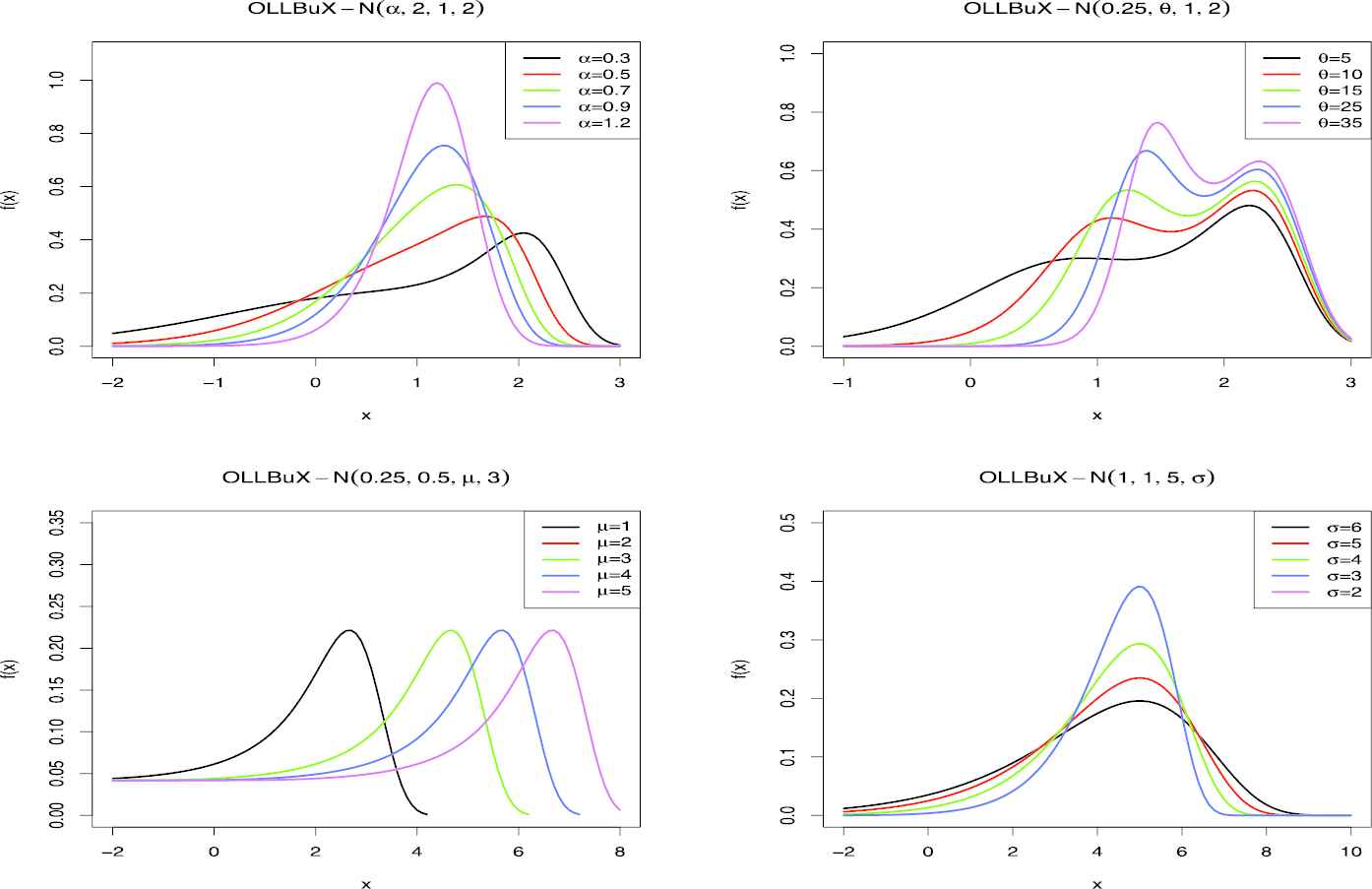
The sample curves of density function of OLLBuX-N(α, θ, μ, σ).
One can see in the curves of Figure 1 that different skewed density functions including mild and high skewed ones (positive and negative) have been produced. The OLLBuX-N family build the very flexible density function (unimodal and bimodal) that is useful in fitting real data sets.
2.2. The OLLBuX-Weibull Family (OLLBuX-W)
By taking
In Figure 2 some density and hazard functions for OLLBuX-W have been drown.
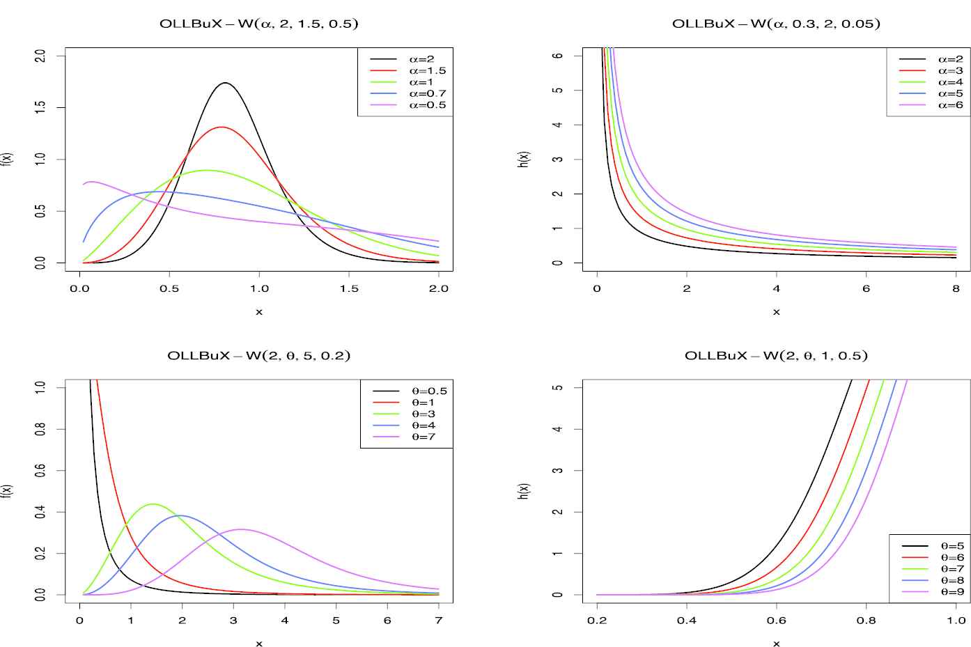
The sample curves of density and hazard function of OLLBuX-W
3. LINEAR COMBINATIONS
Using generalized binomial expansion, for any
Then we can write as the following:
Finally we can write as follows:
4. STATISTICAL PROPERTIES
In this section, we obtain some statistical properties such as: asymptotics, moments, moment-generating function, incomplete moments. Established algebraic expansions to determine some structural properties of the OLLBuX family can be more efficient than computing those directly by numerical integration of its density function.
4.1. Limit Behaviors
Proposition 4.1.1.
Let
Proposition 4.1.2.
The asymptotics of equations F(x), f(x), and h(x), as x → ∞ a are given by the following:
We can evaluate the effect of parameters on tails of distribution using these equations.
4.2. Moments
Henceforth, let
4.3. Moment-Generating Function
The moment-generating function (mgf)
4.4. Incomplete Moments
The nth incomplete moment of X, say
The main applications of the first incomplete moment,
The Lorenz and Bonferroni curves are very useful in economics, reliability, demography, insurance and medicine. For a given probability
5. THE MAXIMUM LIKELIHOOD ESTIMATOR
Several methods for parameter estimation can be used but the maximum likelihood is the most commonly employed. The MLE's enjoy desirable properties to construct confidence intervals for the model parameters. Large sample theory for these estimates delivers simple approximations that work well in finite samples. The commonly used goodness-of-fit statistics to compare fitted models are: the maximum log-likelihood (
Let
The log-likelihood function can be maximized either directly by solving the nonlinear likelihood equations obtained by differentiating (8).
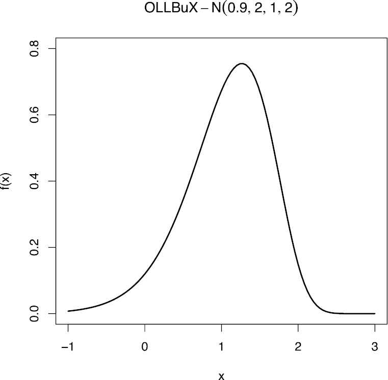
The density function for simulation study.
The components of the score function
6. SIMULATION STUDY
6.1. The Maximum Likelihood Estimator
In this section, the Maximum likelihood estimators of parameters of purpose density function has been assessed by simulating:
To verify the check of the maximum likelihood estimator, the bias of MLE and the mean square error of MLE have been used. For example, as described in Section 5, for
To investigate the performance of the MLE's for the OLLBuX-N distribution, we perform a simulation study:
Generate r samples of size n from Equation (2).
Compute the MLE's for the r samples, say
Compute the standard errors of the MLE's for r samples, say
Compute the biases and mean squared errors given by
andfor
We repeat these steps for r = 1000 and
Figures 4 and 5 respectively reveals how the four biases, mean squared errors vary with respect to n. As expected, the Biases and MSEs of estimated parameters converges to zero while n growing.
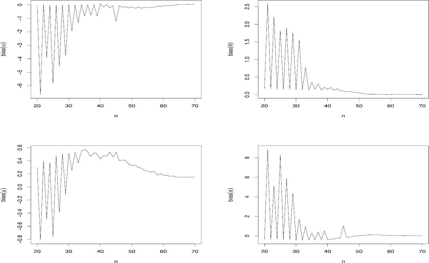
Bias of
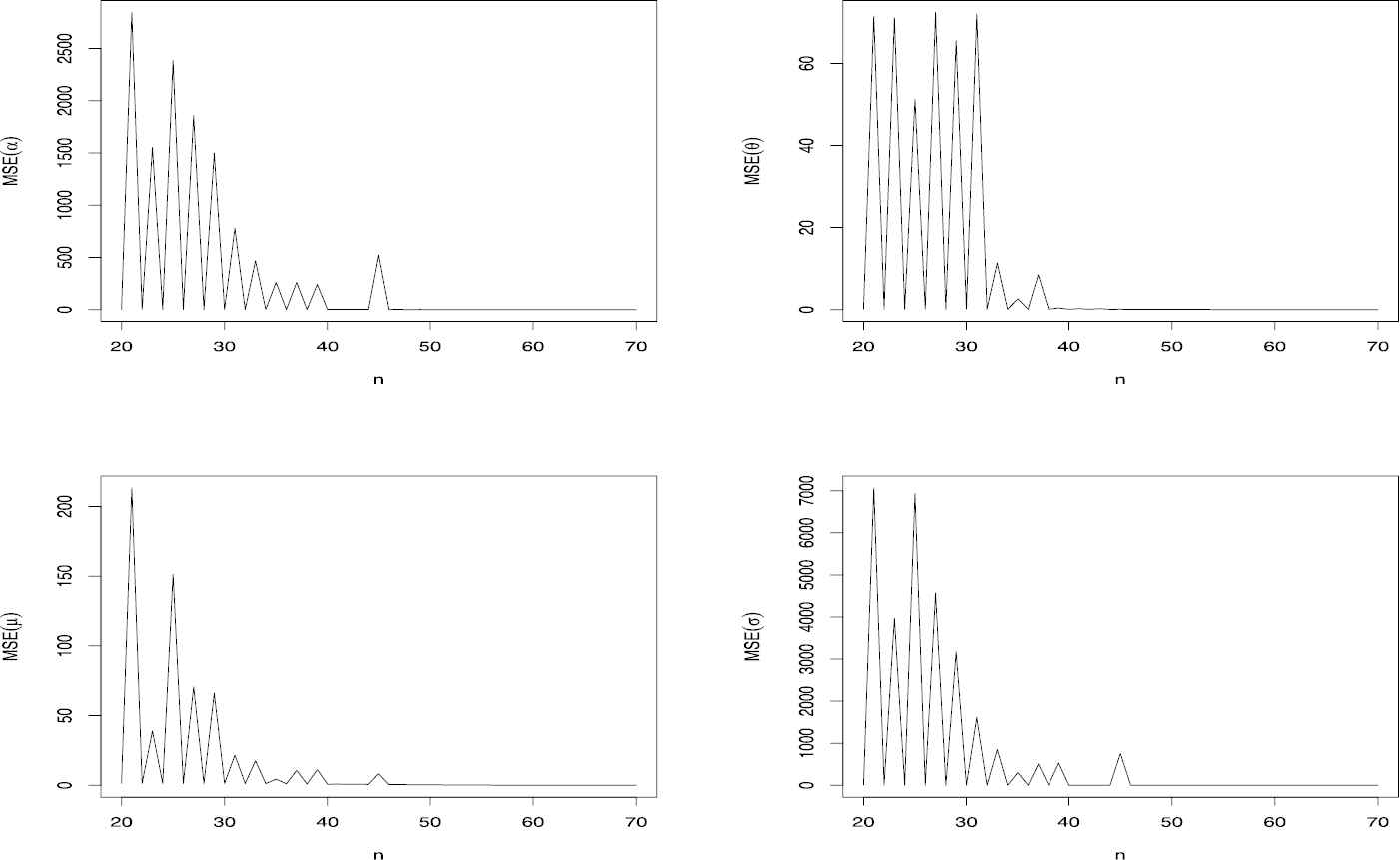
MSE of
6.2. The Other Estimation Methods
There are several approaches to estimate the parameters of distributions that each of them has its characteristic features and benefits. In this subsection five of those methods are briefly introduced and will be numerically investigated in the simulation study Figure 3. A useful summary of these methods can be seen in Dey et al. [16]. Here
6.2.1. Least squares and weighted least squares estimators
The Least Squares (LSE) and weighted Least Squares Estimators (WLSE) are introduced by Swain et al. [17]. The LSE's and WLSE's are obtained by minimizing the following functions:
6.2.2. Cramér–von–Mises estimator
Cramér–von–Mises Estimator (CME) is introduced by Choi and Bulgren [18]. The CMEs is obtained by minimizing the following function:
6.2.3. Anderson–Darling and right-tailed Anderson–Darling
The Anderson Darling (ADE) and Right-Tailed Anderson Darling Estimators (RTADE) are introduced by Anderson and Darling [19]. The ADE's and RTADE's are obtained by minimizing the following functions:
In order to explore the estimators introduced above we consider the one model that have been used in this section, and investigate MSE of those estimators for different samples. For instance according to what has been mentioned above, for
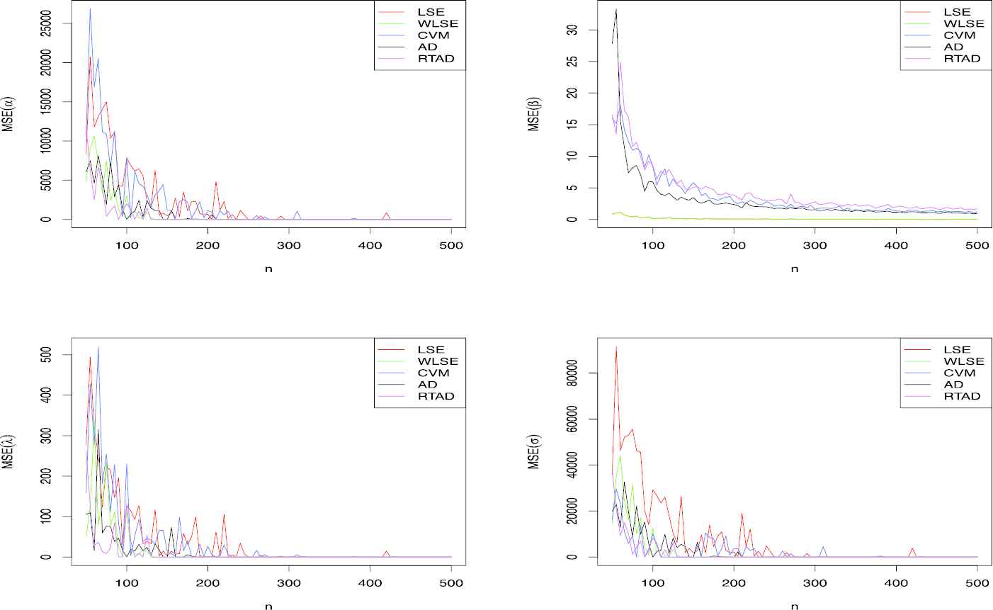
MSE of
7. APPLICATIONS
In this section, we submit two applications by fitting the OLLBuX-N model and some famous models. The AIC, Bayesian information criterion (BIC), Cramér–von Mises (
The gamma-normal distribution (GaN), Alzaatreh et al. [20], The beta-normal distribution (BN), Eugene et al. [6], The McDonald normal distribution (McN), Cordeiro et al. [21], Marshall–Olkin normal distribution (MON), Jose [22], The Kumaraswamy normal distribution (KwN), Cordeiro and de Castro [23], The Zografos–Balakrishnan distribution (ZBN), Nadarajah et al. [24], and Log-normal distribution (LN), have been selected for comparison in the two examples. The parameters of models have been estimated by the MLE method.
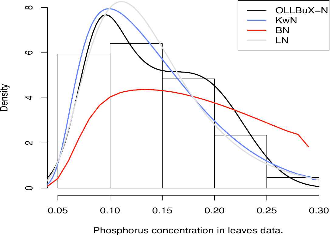
7.1. Phosphorus Concentration in Leaves Data Set
This sub-section is related to study of the soil fertility in influence and the characterization of the biologic fixation of
In the Tables 1 and 2, a summary of the fitted information criteria and estimated MLE's for this data with different models have come, respectively. Models have been sorted from the lowest to the highest value of AIC. As you see, the OLLBuX-N is selected as the best model with more criteria. The histogram of the Phosphorus concentration in leaves data and the plots of fitted pdf are displayed in Figure 7.
| Model | AIC | BIC | K.S | P-Value | ||
|---|---|---|---|---|---|---|
| OLLBuX-N | −393.32 | −381.92 | 0.055 | 0.33 | 0.08 | 0.391 |
| KwN | −388.02 | −376.61 | 0.09 | 0.62 | 0.07 | 0.478 |
| BN | −387.96 | −376.55 | 0.09 | 0.62 | 0.077 | 0.441 |
| LN | −387.94 | −382.24 | 0.13 | 0.82 | 0.082 | 0.35 |
| McN | −386.07 | −371.81 | 0.17 | 0.96 | 0.30 | 0 |
| MON | −381.87 | −373.31 | 0.20 | 1.14 | 0.10 | 0.127 |
| ZBN | −379.47 | −370.91 | 0.41 | 2.75 | 0.946 | 0 |
| Normal | −379.04 | −373.34 | 0.27 | 1.56 | 0.13 | 0.021 |
| GaN | −371.97 | −360.57 | 0.38 | 2.56 | 1 | 0 |
Information criteria for the phosphorus concentration in leaves data.
| Model | MLE | Standard Errors |
|---|---|---|
| OLLBuX-N( |
||
| KwN( |
||
| BN( |
||
| LN( |
||
| McN( |
||
| MON( |
||
| ZBN( |
||
| Normal( |
||
| GaN( |
Estimated MLEs and standard errors for the phosphorus concentration in leaves data.
Histogram for Phosphorus concentration in leaves data set.
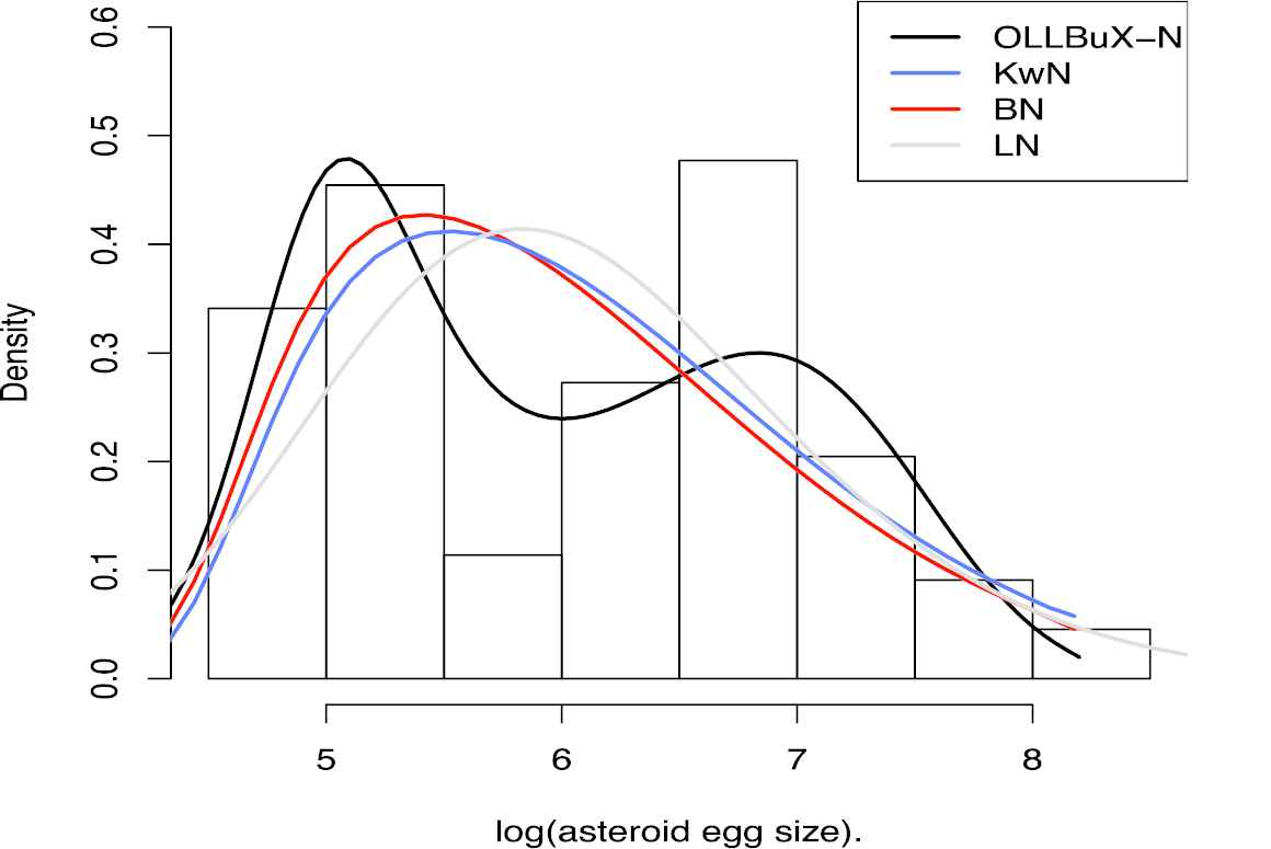
7.2. The Logarithm of the Egg Diameters of the Asteroids Data
This sub-section is related to study of bimodal data set obtained from Emlet et al. [27] on the asteroid and echinoid egg size. The data consists of 88 asteroids species divided into three types; 35 planktotrophic larvae, 36 lecithotrophic larvae and 17 brooding larvae.
The logarithm of the egg diameters of the asteroids data has a bimodal shape.
Similar to the previous application example, we have Tables 3 and 4. As it is clear, the OLLBuX-N is selected as the best model with all criteria.
| Model | AIC | BIC | K.S | P-Value | ||
|---|---|---|---|---|---|---|
| OLLBuX-N | 227.12 | 237.03 | 0.16 | 0.94 | 0.14 | 0.191 |
| KwN | 244.38 | 254.29 | 0.44 | 2.40 | 0.15 | 0.039 |
| BN | 245.26 | 255.17 | 0.44 | 2.42 | 0.17 | 0.0151 |
| LN | 249.56 | 254.51 | 0.46 | 2.62 | 0.16 | 0.021 |
| GaN | 250.48 | 260.39 | 0.57 | 3.27 | 0.19 | 0.003 |
| Normal | 250.74 | 255.69 | 0.40 | 2.42 | 0.17 | 0.01 |
| ZBN | 252.002 | 259.43 | 0.82 | 4.71 | 0.827 | 0 |
| MON | 252.65 | 260.08 | 0.41 | 2.45 | 0.17 | 0.014 |
| McN | 256.22 | 268.61 | 0.42 | 2.48 | 0.91 | 0 |
Information criteria for the logarithm of the egg diameters of the asteroids data.
| Model | MLE | Standard Errors |
|---|---|---|
| OLLBuX-N( |
||
| KwN( |
||
| BN( |
||
| LN( |
||
| GaN( |
||
| Normal( |
||
| ZBN( |
||
| MON( |
||
| McN( |
Estimated MLEs and standard errors of the egg diameters of the asteroids data.
The histogram of the logarithm of the egg diameters of the asteroids data and the plots of fitted pdf are displayed in Figure 8.
Histogram for the logarithm of the egg diameters of the asteroids data.
8. CONCLUSIONS
A new class of distributions called the OLL Burr-X family with two extra positive parameters is introduced and studied. The new generator extends the OLL and Burr X distributions among several other well-known distributions. We provide some mathematical properties of the new family including moments and incomplete moments and generating function. Different methods have been used to estimate its parameters such as maximum likelihood, Least squares, weighted least squares, Cramer–von-Mises, Anderson–Darling and right-tailed Anderson–Darling methods. We assesses the performance of the maximum likelihood estimators in terms of biases and mean squared errors by means of a simulation study. Finally, the usefulness of the family is illustrated by means of two real data sets. The new models provide consistently better fits than other competitive models for these data sets. The new family is suitable for fitting different real data sets, the OLL Burr-X normal model is used for modeling bimodal and skewed data sets and can be sued as an alternative to the gamma-normal, beta-normal, McDonald-normal, Marshall-Olkin-normal, Kumaraswamy-normal, Zografos-Balakrishnan and log-normal distributions.
CONFLICTS OF INTEREST
The authors declare they have no conflicts of interest.
AUTHORS' CONTRIBUTIONS
The authors have equally made contributions. All authors read and approved the final manuscript.
ACKNOWLEDGMENTS
The authors greatly appreciate both the Editor-in-Chief and the referees. This research is supported by Research Committee of Persian Gulf University.
REFERENCES
Cite this article
TY  - JOUR
AU  - Hamid Karamikabir
AU  - Mahmoud Afshari
AU  - Morad Alizadeh
AU  - Haitham M. Yousof
PY  - 2021
DA  - 2021/06/15
TI  - The Odd Log-Logistic Burr-X Family of Distributions: Properties and Applications
JO  - Journal of Statistical Theory and Applications
SP  - 228
EP  - 241
VL  - 20
IS  - 2
SN  - 2214-1766
UR  - https://doi.org/10.2991/jsta.d.210609.001
DO  - 10.2991/jsta.d.210609.001
ID  - Karamikabir2021
ER  -