
Progressively Censored N-H Exponential Distribution
- DOI
- 10.2991/jsta.d.210322.002How to use a DOI?
- Keywords
- Progressive type II censoring samples; Maximum likelihood estimation; Bayesian estimation; Lindely's approximation; Gibbs sampling
- Abstract
An extended version of exponential distribution is considered in this paper. This lifetime distribution has increasing, decreasing and constant hazard rates. So it can be considered as another useful two-parameter extension/generalization of the exponential distribution. It can be used as an alternative to the gamma, Weibull and exponentiated exponential distributions. Maximum likelihood and Bayes estimates for two parameter of N-H exponential distribution are obtained based on a progressive type II censored samples. Bayesian estimates are obtained using squared error loss function. These Bayesian estimates are evaluated by applying the Lindely's approximation method.
- Copyright
- © 2021 The Authors. Published by Atlantis Press B.V.
- Open Access
- This is an open access article distributed under the CC BY-NC 4.0 license (http://creativecommons.org/licenses/by-nc/4.0/).
1. INTRODUCTION
The exponential distribution is a popular choices for analyzing lifetime data, but the constant hazard rate makes it not suited in several practical situations. In such situations the Weibull and gamma models are frequently employed. The either increasing or decreasing hazard rate of these distributions marked them unfit for the analysis of many lifetime data sets where the hazard rate is U-shaped. This led some authors to introduce extensions or generalization of the exponential distribution as alternative models. In [1] Gupta and Kundu introduced the exponentiated (or generalized) exponential distribution and in [2] Nadarajah and Kotz introduced a generalization of exponential distribution referred to as the beta exponential distribution which is generated from the logit of a beta random variable. Also, Gupta and Kundu [3] introduced a shape parameter to an exponential model using the idea of Azzalini and called it weighted exponential distribution. Nadarajah and Haghighi [4] introduced another extension of the exponential distribution which was later called the N-H exponential distribution. Here, we will be concerned with the N-H exponential distribution. This distribution has survival function given by
The corresponding cdf, pdf and hazard function are given by
The conventional type I and type II censoring allow for units to be removed or lost from the test at prefixed time and prefixed no of failures, respectively. These types of censoring are common censoring schemes but they do not have the facility of allowing removal of units at points other than the terminal points of the test. In this article a progressive sample scheme as popularized by [5], in particular progressive type II right censoring scheme will be considered.
Under progressive type II right censoring scheme, n units are placed on a test at time 0. At the first failure,
In this paper, we discuss the mle of the two unknown parameters of N-H exponential with approximate confidence interval under progressive type II right censoring.
2. MAXIMUM LIKELIHOOD ESTIMATION
Suppose we have
Differentiating Equation (7) with respect to
Solving Equations (8) and (9), we obtain
3. BAYESIAN ESTIMATION
Now we will discuss parameter estimation via Bayesian viewpoint. Assuming that the two parameters
respectively. Two reasons for choosing gamma priors; one is its mathematical tractability and the other is due to the fact that if we known from experience some information about the parameter of interest, like its mean and its variance, it would be fairly easy to calculate the hyper-parameters of the gamma priors. The joint prior distribution for
The joint posterior distribution of
Therefore, the Bayes estimate of any function of
It is not easy to compute this integral, so one can use one of the approximation methods such as Lindely's approximation. Using this method we have the approximate Bayes estimate of
4. A NUMERICAL STUDY
Here, we present some numerical results to show the behavior of the proposed method for various sample sizes (n = 20, 25, 30, 50, 70, 100); different effective sample sizes(m = 5, 10, 15, 20, 25, 30, 50); two different priors (noninformative prior and informative prior); two different censoring schemes (details of the schemes are given in Tables 1 and 2).
| n | m | R1,…,Rm | Scheme Number |
|---|---|---|---|
| 20 | 5 | (3 * 5)a | [1] |
| (5, 0, 5, 0, 5) | [2] | ||
| (0, 5, 2, 5, 3) | [3] | ||
| (0 * 4, 15) | [4] | ||
| 20 | 10 | (1 * 2, 0, 2 * 2, 0, 2, 1 * 2) | [5] |
| (10, 0 * 9) | [6] | ||
| (0 * 9, 10) | [7] | ||
| (2 * 2, 0 * 2, 0 * 3, 2 * 2) | [8] | ||
| 25 | 10 | (2 * 2, 0 * 2, 1 * 4, 5, 2) | [9] |
| (0 * 5, 5 * 3, 0 * 2) | [10] | ||
| (1 * 4, 2 * 3, 0 * 2, 5) | [11] | ||
| (0 * 4, 15, 0 * 5) | [12] | ||
| 25 | 15 | (1, 2, 0 * 2, 1, 2, 0 * 3, 1, 0 * 3, 2) | [13] |
| (0 * 10, 2 * 5) | [14] | ||
| (1 * 10, 0 * 5) | [15] | ||
| (1 * 5, 0 * 5, 1 * 5) | [16] | ||
| 30 | 15 | (0 * 14, 15) | [17] |
| (1 * 10, 0 * 4, 5) | [18] | ||
| (0 * 5, 1 * 5, 2 * 5) | [19] | ||
| (2 * 5, 0 * 9, 5) | [20] | ||
| 30 | 20 | (3, 0 * 4, 3, 0 * 4, 1, 0 * 4) | [21] |
| (1 * 10, 0 * 10) | [22] | ||
| (1 * 5, 0 * 5, 1 * 5, 0 * 5) | [23] | ||
| (2 * 5, 0 * 15) | [24] | ||
| 50 | 20 | (1 * 5, 0 * 14, 25) | [25] |
| (10, 0 * 4, 1 * 10, 2 * 5) | [26] | ||
| (0 * 5, 2 * 10, 0 * 3, 5 * 2) | [27] | ||
| (1 * 10, 0 * 5, 5 * 4) | [28] | ||
| 50 | 25 | (0 * 5, 1 * 5, 0 * 5, 2 * 3, 3 * 2, 4 * 2, 0 * 3) | [29] |
| (1 * 25) | [30] | ||
| (0 * 24, 25) | [31] | ||
| (1 * 5, 0 * 16, 4 * 5) | [32] | ||
| 100 | 30 | (2 * 5, 0 * 5, 5 * 5, 0 * 5, 6 * 5, 1 * 5) | [33] |
| (0 * 10, 2 * 10, 0 * 5, 10 * 5) | [34] | ||
| (5 * 5, 0 * 20, 9 * 5) | [35] | ||
| (2 * 5, 0 * 5, 10 * 5, 0 * 5, 2 * 5) | [36] | ||
| 100 | 50 | (0 * 15, 1 * 5, 0 * 5, 5 * 5, 0 * 15, 4 * 5) | [37] |
| (2 * 5, 1 * 10, 0 * 10, 5 * 5, 0 * 15, 1 * 5) | [38] | ||
| (0 * 35, 5 * 5, 0 * 5, 5 * 5) | [39] | ||
| (2 * 10, 0 * 20, 1 * 10, 2 * 20) | [40] |
(a) This 3 * 5 denotes that 3, 3, 3, 3, 3. This table is adapted from Dey and Dey [6].
Different censoring schemes for the simulation study.
| n | m | R1,…,Rm | Scheme Number |
|---|---|---|---|
| 20 | 5 | (1, 4, 1 * 3a) | [1] |
| (4, 1, 2 * 2, 3) | [2] | ||
| (1, 0, 2, 5 * 2) | [3] | ||
| (2, 1, 3 * 3) | [4] | ||
| (2, 1, 4, 3 * 2) | [5] | ||
| (2, 4, 9, 5, 3) | [6] | ||
| 50 | 5 | (1, 4, 1 * 3) | [7] |
| (4, 1, 2 * 2, 3) | [8] | ||
| (1, 0, 2, 5 * 2) | [9] | ||
| (2, 1, 3 * 3) | [10] | ||
| (2, 1, 4, 3 * 2) | [11] | ||
| (2, 4, 9, 5, 3) | [12] | ||
| 50 | 10 | (1, 5, 1, 3, 2, 1, 3, 0, 3 * 2) | [13] |
| (1, 8, 5, 1, 4 * 4, 2, 4) | [14] | ||
| (3, 2, 5, 2, 3, 4, 2, 1, 3, 4) | [15] | ||
| (1, 3, 6, 0 * 2, 6, 2, 3, 2, 0) | [16] | ||
| (4, 3, 1, 2, 1, 2, 1 * 2, 2, 6) | [17] | ||
| (4, 1, 3, 5, 4, 7, 2, 5, 3, 1) | [18] | ||
| 70 | 10 | (1, 8, 5, 1, 4 * 4, 2, 4) | [19] |
| (1, 8, 5, 1, 4 * 4, 2, 4) | [20] | ||
| (3, 2, 5, 2, 3, 4, 2, 1, 3, 4) | [21] | ||
| (1, 3, 6, 0 * 2, 6, 2, 3, 2, 0) | [22] | ||
| (4, 3, 1, 2, 1, 2, 1 * 2, 2, 6) | [23] | ||
| (4, 1, 3, 5, 4, 7, 2, 5, 3, 1) | [24] | ||
| 70 | 15 | (1, 3, 0 * 2, 3, 2, 3 * 2, 2, 1, 2 * 2, 1, 3, 2) | [25] |
| (2, 3 * 2, 4 * 3, 1, 3, 0, 2 * 2, 3, 1, 5, 1) | [26] | ||
| (2, 3 * 2, 4 * 2, 1, 0, 2, 3 * 2, 2, 4 * 3, 5) | [27] | ||
| (5, 3 * 2, 1, 2, 5, 4 * 2, 1, 3, 2, 3, 4, 2, 1) | [28] | ||
| (4, 1, 4, 3, 6, 3, 2, 1, 3, 4, 2 * 2, 7, 1, 2) | [29] | ||
| (1, 5, 2, 5, 1, 3, 6, 2, 4, 3, 5, 4, 1, 6, 3) | [30] | ||
| 100 | 15 | (1, 3, 0 * 2, 3, 2, 3 * 2, 2, 1, 2 * 2, 1, 3, 2) | [31] |
| (2, 3 * 2, 4 * 3, 1, 3, 0, 2 * 2, 3, 1, 5, 1) | [32] | ||
| (2, 3 * 2, 4 * 2, 1, 0, 2, 3 * 2, 2, 4 * 3, 5) | [33] | ||
| (5, 3 * 2, 1, 2, 5, 4 * 2, 1, 3, 2, 3, 4, 2, 1) | [34] | ||
| (4, 1, 4, 3, 6, 3, 2, 1, 3, 4, 2 * 2, 7, 1, 2) | [35] | ||
| (1, 5, 2, 5, 1, 3, 6, 2, 4, 3, 5, 4, 1, 6, 3) | [36] | ||
| 100 | 20 | (4, 5, 2 * 2, 1, 4, 2, 1, 4, 5 * 2, 4, 3, 2, 5, 3, 1, 6, 1, 3) | [37] |
| (5, 3, 1, 3, 4 * 2, 3 * 2, 0, 3 * 2, 1 * 2, 5, 4, 2, 3, 5, 6, 2) | [38] | ||
| (1, 4, 2, 3, 5 * 2, 6, 3 * 2, 1, 3, 5, 3, 4, 3, 2 * 2, 4, 6, 3) | [39] | ||
| (4, 2, 4, 2, 1, 9, 3, 5, 4, 2, 5, 1, 3, 5, 6, 3, 4 * 2, 1 * 2) | [40] | ||
| (3, 4, 2, 1, 2, 5, 4, 6, 2, 4, 2 * 2, 0, 2 * 2, 6, 2, 1, 3 * 2) | [41] | ||
| (1 * 2, 4, 3 * 2, 7, 2, 1, 2 * 3, 0, 3 * 2, 2 * 2, 4, 2, 3) | [42] |
(a) This 1 * 3 denotes that 1, 1, 1.
Different censoring schemes from poisson with mean 3 for the simulation study.
For
| Prior 0 |
Prior 1 |
||||
|---|---|---|---|---|---|
| n | m | Scheme | |||
| 20 | 5 | [1] | 0.4971915(0.528149) | 0.4971415(0.528073) | 0.4971915(0.528037) |
| [2] | 0.4829925(0.514042) | 0.4829210(0.513973) | 0.4829030(0.513955) | ||
| [3] | 0.5218350(0.539559) | 0.5217500(0.539468) | 0.5217300(0.539450) | ||
| [4] | 0.5191600(0.548442) | 0.5190850(0.548365) | 0.5190650(0.548347) | ||
| 20 | 10 | [5] | 0.3415230(0.319913) | 0.3415040(0.319884) | 0.3414970(0.319880) |
| [6] | 0.2649890(0.242477) | 0.2649600(0.242462) | 0.2649545(0.242459) | ||
| [7] | 0.2499280(0.204724) | 0.2498940(0.204707) | 0.2498885(9.204704) | ||
| [8] | 0.3022270(0.282316) | 0.3021885(0.282293) | 0.3021795(0.282287) | ||
| 25 | 10 | [9] | 0.3588315(0.324342) | 0.3587875(0.324310) | 0.3587775(0.324303) |
| [10] | 0.3572780(0.335403) | 0.3572250(0.335365) | 0.3572175(0.335360) | ||
| [11] | 0.3200430(0.293386) | 0.3199970(0.293357) | 0.3199845(0.293349) | ||
| [12] | 0.3178110(0.324944) | 0.3178705(0.324918) | 0.3178645(0.324915) | ||
| 25 | 15 | [13] | 0.1958475(0.150822) | 0.1958060(0.150805) | 0.1957970(0.150802) |
| [14] | 0.2375360(0.188130) | 0.2374980(0.188111) | 0.2374890(0.188107) | ||
| [15] | 0.2051600(0.158191) | 0.2051200(0.158175) | 0.2051120(0.158171) | ||
| [16] | 0.2297045(0.180323) | 0.2296675(0.180306) | 0.2296595(0.180303) | ||
| 30 | 15 | [17] | 0.6506570(0.556114) | 0.6505650(0.555973) | 0.6505600(0.555970) |
| [18] | 0.6489950(0.565434) | 0.648880(0.565299) | 0.648880(0.565297) | ||
| [19] | 0.2339490(0.191414) | 0.2339100(0.191396) | 0.2338995(0.191391) | ||
| [20] | 0.2132375(0.167186) | 0.2131960(0.167168) | 0.2131865(0.167164) | ||
| 30 | 20 | [21] | 0.1545180(0.103939) | 0.1544675(0.103924) | 0.1544590(0.103921) |
| [22] | 0.1380175(0.092865) | 0.1379555(0.0902693) | 0.1379460(0.0902667) | ||
| [23] | 0.1512940(0.101957) | 0.1512420(0.101942) | 0.1512330(0.101939) | ||
| [24] | 0.1240075(0.0777336) | 0.1239540(0.0777203) | 0.1239440(0.0777178) | ||
| 50 | 20 | [25] | 0.2211845(0.164537) | 0.2211475(0.164521) | 0.2211360(0.164516) |
| [26] | 0.2100615(0.156362) | 0.2100215(0.156345) | 0.210012(0.156341) | ||
| [27] | 0.1987010(0.155447) | 0.1986630(0.155431) | 0.1986510(0.155427) | ||
| [28] | 0.2080380(0.157063) | 0.208000(0.157047) | 0.2079890(0.157042) | ||
| 50 | 25 | [29] | 0.1816730(0.125538) | 0.1816190(0.125518) | 0.1816090(0.125514) |
| [30] | 0.1649060(0.110223) | 0.1648620(0.110209) | 0.1648530(0.110206) | ||
| [31] | 0.1656070(0.121050) | 0.1655740(0.121040) | 0.1655630(0.121036) | ||
| [32] | 0.1638900(0.112809) | 0.1638530(0.112797) | 0.1638420(0.112793) | ||
| 100 | 30 | [33] | 0.1778810(0.119835) | 0.1778280(0.119816) | 0.1778150(0.119812) |
| [34] | 0.1483560(0.114650) | 0.1483260(0.114641) | 0.1483120(0.114637) | ||
| [35] | 0.1623790(0.116393) | 0.1623460(0.116382) | 0.1623330(0.116378) | ||
| [36] | 0.1595940(0.112488) | 0.1595460(0.112472) | 0.1595330(0.112468) | ||
| 100 | 50 | [37] | 0.0976598(0.0564262) | 0.0976067(0.0564159) | 0.097594(0.0564135) |
| [38] | 0.0736086(0.0384041) | 0.0734818(0.0383854) | 0.0734641(0.0383828) | ||
| [39] | 0.0942280(0.0610751) | 0.0941882(0.061076) | 0.0941766(0.0610654) | ||
| [40] | 0.0857108(0.04392267) | 0.0856541(0.048214) | 0.0856418(0.0439158) |
mle, maximum likelihood estimation.
The absolute value of bias and the mean squared error for the mle and Bayes estimates of
| Prior 0 |
Prior 1 |
||||
|---|---|---|---|---|---|
| n | m | Scheme | |||
| 20 | 5 | [1] | 0.1159850(2.440330) | 0.1159210(2.440330) | 0.1159860(2.440330) |
| [2] | 0.1664680(2.877200) | 0.1663370(2.877670) | 0.1664760(2.877720) | ||
| [3] | 0.0521421(2.208430) | 0.0520099(2.208420) | 0.0521356(2.208430) | ||
| [4] | 0.1428650(2.925990) | 0.1427380(2.925950) | 0.1428660(2.925990) | ||
| 20 | 10 | [5] | 0.0468047(1.475010) | 0.0468103(1.475010) | 0.4672770(1.475010) |
| [6] | 0.1489790(1.847030) | 0.1489070(1.847010) | 0.1490000(1.847040) | ||
| [7] | 0.0996390(1.687940) | 0.0995607(1.687920) | 0.0996578(1.687940) | ||
| [8] | 0.1553390(1.709930) | 0.1552530(1.709900) | 0.1553590(1.709930) | ||
| 25 | 10 | [9] | 0.1151180(1.894140) | 0.1150350(1.894120) | 0.1151330(1.894140) |
| [10] | 0.00097442(1.27014) | 0.0097176(1.27014) | 0.00980259(1.27014) | ||
| [11] | 0.1550760(1.930400) | 0.1549820(1.930370) | 0.1551000(1.930400) | ||
| [12] | 0.0614795(1.129176) | 0.0614042(1.29176) | 0.0614893(1.29177) | ||
| 25 | 15 | [13] | 0.1042340(1.083920) | 0.1041470(1.083910) | 0.1042640(1.083930) |
| [14] | 0.0970686(1.266200) | 0.0969918(1.266180) | 0.0970923(1.266200) | ||
| [15] | 0.0998006(1.173930) | 0.0997249(1.173910) | 0.0998328(1.173930) | ||
| [16] | 0.0980328(1.323670) | 0.0979575(1.323650) | 0.0980556(1.323670) | ||
| 30 | 15 | [17] | 0.2909370(0.592421) | 0.2909970(0.592457) | 0.2909670(0.592439) |
| [18] | 0.2861400(0.628215) | 0.2861990(0.628249) | 0.2861690(0.628232) | ||
| [19] | 0.1142530(1.281150) | 0.1151730(1.281130) | 0.1152810(1.281150) | ||
| [20] | 0.1052180(1.131820) | 0.1051320(1.131800) | 0.1052460(1.131820) | ||
| 30 | 20 | [21] | 0.0397746(0.722620) | 0.0396972(0.722614) | 0.0398096(0.722623) |
| [22] | 0.0163531(0.645947) | 0.0162683(0.645945) | 0.0163926(0.645949) | ||
| [23] | 0.0528775(0.718214) | 0.0527984(0.718206) | 0.0529175(0.718278) | ||
| [24] | 0.0919885(0.879429) | 0.0919003(0.879413) | 0.0920422(0.879439) | ||
| 50 | 20 | [25] | 0.1060660(1.094770) | 0.1059960(1.094750) | 0.1060980(1.094770) |
| [26] | 0.0639464(0.918429) | 0.0638751(0.918420) | 0.0639725(0.918433) | ||
| [27] | 0.1027290(1.003060) | 0.1026540(1.003050) | 0.1027620(1.003070) | ||
| [28] | 0.0921558(0.996051) | 0.0920827(0.996037) | 0.092190(0.996057) | ||
| 50 | 25 | [29] | 0.0226088(0.513429) | 0.0226722(0.513432) | 0.0225785(0.513428) |
| [30] | 0.0412888(0.746001) | 0.0412199(0.745995) | 0.0413179(0.746004) | ||
| [31] | 0.1573980(1.070030) | 0.1573300(1.070010) | 0.1574360(1.070050) | ||
| [32] | 0.0939640(0.882445) | 0.0938659(0.882432) | 0.0939705(0.882451) | ||
| 100 | 30 | [33] | 0.0221276(0.492459) | 0.0221921(0.462462) | 0.0220961(0.492458) |
| [34] | 0.1468470(0.877965) | 0.1467860(0.877947) | 0.1468920(0.877978) | ||
| [35] | 0.1084710(0.777371) | 0.1084100(0.777358) | 0.1085090(0.777379) | ||
| [36] | 0.0209500(0.707031) | 0.0208773(0.707029) | 0.0209798(0.499895) | ||
| 100 | 50 | [37] | 0.0221536(0.365813) | 0.0220891(0.365810) | 0.0221887(0.365815) |
| [38] | 0.00189239(0.266265) | 0.00180332(0.266265) | 0.00195382(0.266265) | ||
| [39] | 0.0798200(0.450539) | 0.0797579(0.450530) | 0.7985540(0.450545) | ||
| [40] | 0.0351824(0.391901) | 0.0351142(0.0482149) | 0.0352210(0.391903) |
mle, maximum likelihood estimation.
The absolute value of bias and the mean squared error for the mle and Bayes estimates of
| Prior 0 |
Prior 1 |
||||
|---|---|---|---|---|---|
| n | m | Scheme | |||
| 20 | 5 | [1] | 0.3264670(0.174211) | 0.3263265(0.174119) | 0.326554(0.174268) |
| [2] | 0.3125085(0.175525) | 0.3109845(0.174575) | 0.3107235(0.174413) | ||
| [3] | 0.2932695(0.156102) | 0.2928570(0.155861) | 0.2927425(0.155793) | ||
| [4] | 0.2964170(0.165958) | 0.2951265(0.165194) | 0.2948700(0.165043) | ||
| [5] | 0.3033180(0.170888) | 0.3027190(0.170527) | 0.3025795(0.170442) | ||
| [6] | 0.3056350(0.171403) | 0.3053230(0.171213) | 0.3052520(0.171169) | ||
| 50 | 5 | [7] | 0.2326710(0.104817) | 0.2326680(0.104816) | 0.2328510(0.104901) |
| [8] | 0.227333(0.0996646) | 0.227330(0.0996633) | 0.227517(0.0997482) | ||
| [9] | 0.2312230(0.101513) | 0.2312220(0.101512) | 0.2314180(0.101603) | ||
| [10] | 0.2448950(0.108718) | 0.2448930(0.108717) | 0.2450840(0.108810) | ||
| [11] | 0.2361100(0.102681) | 0.2361080(0.102681) | 0.2362990(0.102771) | ||
| [12] | 0.2281270(0.102811) | 0.2281250(0.102811) | 0.2283180(0.102899) | ||
| 50 | 10 | [13] | 0.2023535(0.098225) | 0.2023340(0.098217) | 0.2024420(0.098261) |
| [14] | 0.2194495(0.113864) | 0.2189520(0.113646) | 0.2188260(0.113591) | ||
| [15] | 0.1995715(0.100056) | 0.1993410(0.0999638) | 0.1995460(0.100046) | ||
| [16] | 0.188810(0.0991293) | 0.1887925(0.0991227) | 0.188901(0.0991636) | ||
| [17] | 0.1891650(0.0951523) | 0.1891255(0.0951374) | 0.1892485(0.0951839) | ||
| [18] | 0.2115465(0.107693) | 0.164785(0.0900948) | 0.162992(0.0895071) | ||
| 70 | 10 | [19] | 0.196174(0.0991527) | 0.196152(0.0991441) | 0.196262(0.0991872) |
| [20] | 0.2076240(0.109312) | 0.2071970(0.109135) | 0.2070780(0.109086) | ||
| [21] | 0.1925230(0.0981574) | 0.1923310(0.0980836) | 0.1925220(0.0981572) | ||
| [22] | 0.178040(0.0892947) | 0.178025(0.0892892) | 0.178025(0.0892892) | ||
| [23] | 0.181694(0.0942027) | 0.181657(0.0941896) | 0.181779(0.0942337) | ||
| [24] | 0.2236670(0.113502) | 0.1999880(0.103470) | 0.1987630(0.102982) | ||
| 70 | 15 | [25] | 0.1525525(0.074663) | 0.1525445(0.0746605) | 0.1526105(0.0746808) |
| [26] | 0.1610365(0.078941) | 0.160040(0.0789305) | 0.161088(0.0789577) | ||
| [27] | 0.1604285(0.0792977) | 0.1594515(0.0789853) | 0.159724(0.0790723) | ||
| [28] | 0.153904(0.0788255) | 0.153777(0.0787864) | 0.159724(0.0790723) | ||
| [29] | 0.160811(0.0844711) | 0.160308(0.0843096) | 0.1605155(0.0843761) | ||
| [30] | 0.173772(0.0840183) | 0.1730975(0.0837843) | 0.172953(0.0837344) | ||
| 100 | 15 | [31] | 0.131363(0.0640767) | 0.131362(0.0640763) | 0.131421(0.0640919) |
| [32] | 0.137894(0.0678622) | 0.137892(0.0678616) | 0.137954(0.0678788) | ||
| [33] | 0.127235(0.0637183) | 0.127232(0.0637175) | 0.127301(0.245602) | ||
| [34] | 0.140579(0.068427) | 0.140577(0.0684264) | 0.140641(0.0684443) | ||
| [35] | 0.142327(0.0668081) | 0.142325(0.0668075) | 0.142389(0.0668256) | ||
| [36] | 0.133757(0.0670613) | 0.133751(0.0670596) | 0.133827(0.0670801) | ||
| 100 | 20 | [37] | 0.619528(0.061622) | 0.115463(0.0616065) | 0.1195515(0.0616277) |
| [38] | 0.124516(0.0623036) | 0.124466(0.0622911) | 0.124598(0.0632512) | ||
| [39] | 0.133008(0.0679955) | 0.1322985(0.0678074) | 0.132512(0.0678639) | ||
| [40] | 0.137380(0.0704051) | 0.1368745(0.0702666) | 0.1370595(0.0703172) | ||
| [41] | 0.139426(0.0687665) | 0.1394075(0.0687612) | 0.139470(0.0687788) | ||
| [42] | 0.120810(0.0583184) | 0.1207935(0.0583143) | 0.120857(0.0583296) |
mle, maximum likelihood estimation.
The average bias and the mean squared error for the mle and Bayes estimates of
| Prior 0 |
Prior 1 |
||||
|---|---|---|---|---|---|
| n | m | Scheme | |||
| 20 | 5 | [1] | 0.1450170(0.414535) | 0.1539360(0.414510) | 0.1540930(0.414558) |
| [2] | 0.1222220(0.595943) | 0.1225950(0.596034) | 0.1221080(0.595915) | ||
| [3] | 0.0959207(0.553236) | 0.0961172(0.553274) | 0.0958474(0.553222) | ||
| [4] | 0.0977636(0.500359) | 0.0981262(0.500431) | 0.9762980(0.500333) | ||
| [5] | 0.1127710(0.486695) | 0.1130020(0.486747) | 0.1126970(0.486678) | ||
| [6] | 0.1295870(0.516272) | 0.1297450(0.516313) | 0.1295510(0.516263) | ||
| 50 | 5 | [7] | 0.0638504(0.339343) | 0.3393430(0.582532) | 0.3393460(0.582534) |
| [8] | 0.0764455(0.305708) | 0.0764358(0.305706) | 0.0764867(0.305714) | ||
| [9] | 0.0891549(0.300518) | 0.0891353(0.300515) | 0.0892121(0.300528) | ||
| [10] | 0.0753222(0.338732) | 0.0753097(0.338730) | 0.0753691(0.338739) | ||
| [11] | 0.0953258(0.298049) | 0.0953122(0.298046) | 0.0953706(0.298057) | ||
| [12] | 0.0628087(0.316734) | 0.0627925(0.316732) | 0.0628660(0.316741) | ||
| 50 | 10 | [13] | 0.0846792(0.362508) | 0.0846487(0.362503) | 0.0847311(0.362517) |
| [14] | 0.0865706(0.407572) | 0.0867438(0.407602) | 0.0864742(0.407556) | ||
| [15] | 0.0345237(0.423932) | 0.0344032(0.423924) | 0.0346810(0.423943) | ||
| [16] | 0.0276860(0.386191) | 0.0276545(0.386189) | 0.0277470(0.386194) | ||
| [17] | 0.0441424(0.396225) | 0.0440963(0.396221) | 0.0442209(0.396232) | ||
| [18] | 0.0894087(0.389970) | 0.0906514(0.390193) | 0.0876544(0.389659) | ||
| 70 | 10 | [19] | 0.0660680(0.390865) | 0.0665740(0.390660) | 0.0666644(0.390872) |
| [20] | 0.0429737(0.465414) | 0.0431430(0.465429) | 0.0428696(0.465405) | ||
| [21] | 0.0507068(0.369911) | 0.0505973(0.369900) | 0.050848(0.369926) | ||
| [22] | 0.0436478(0.369652) | 0.0436186(0.369650) | 0.0436186(0.369650) | ||
| [23] | 0.0342054(0.389776) | 0.0341602(0.389773) | 0.0342852(0.389782) | ||
| [24] | 0.0115685(0.376568) | 0.116635(0.376789) | 0.114665(0.376333) | ||
| 70 | 15 | [25] | 0.0297971(0.305182) | 0.0297808(0.305181) | 0.0298339(0.305185) |
| [26] | 0.0550084(0.316372) | 0.0549709(0.312447) | 0.0550635(0.316378) | ||
| [27] | 0.0591451(0.335305) | 0.0589468(0.335281) | 0.0593916(0.335334) | ||
| [28] | 0.0193960(0.368465) | 0.0193132(0.368462) | 0.0194974(0.368469) | ||
| [29] | 0.0209317(0.381710) | 0.0207688(0.381703) | 0.0211117(0.381718) | ||
| [30] | 0.0646878(0.324553) | 0.0648706(0.324577) | 0.0645641(0.324537) | ||
| 100 | 15 | [31] | 0.0003732(0.322194) | 0.0003785(0.322194) | 0.0003493(0.322194) |
| [32] | 0.0004736(0.349041) | 0.0004647(0.349041) | 0.0005050(0.349041) | ||
| [33] | 0.0138877(0.300106) | 0.0139039(0.300106) | 0.0138432(0.300105) | ||
| [34] | 0.0322061(0.284619) | 0.0321953(0.284618) | 0.0322364(0.284621) | ||
| [35] | 0.0390078(0.288319) | 0.0389973(0.288319) | 0.0390370(0.288322) | ||
| [36] | 0.0073213(0.341275) | 0.00734502(0.341275) | 0.0072675(0.341274) | ||
| 100 | 20 | [37] | 0.0123209(0.296028) | 0.0122654(0.296027) | 0.0123992(0.296030) |
| [38] | 0.0273074(0.271238) | 0.0272604(0.271235) | 0.0273765(0.271241) | ||
| [39] | 0.0186184(0.311621) | 0.0184501(0.311615) | 0.0188311(0.311629) | ||
| [40] | 0.0037491(0.355722) | 0.0035876(0.355721) | 0.0039160(0.355723) | ||
| [41] | 0.0386721(0.294793) | 0.0386447(0.294791) | 0.0387159(0.294796) | ||
| [42] | 0.0168828(0.269872) | 0.0168550(0.269871) | 0.0169318(0.269874) |
mle, maximum likelihood estimation.
The average bias and the mean squared error for the mle and Bayes estimates of
From Tables 4–6, one can note that for fixed sample size n, as effective sample size m increases, the implementations improve in terms of bias and MSEs in both procedures. Bayes estimates under Lindely's method is similar to the mle estimates as expected. In case of Bayes estimates, the results of Prior0 is similar to Prior1.
5. A CASE OF REAL DATA
The data set in Table 7 represents the remission times (in months) of a sample of size 128 bladder cancer patients reported in [8]. The plot in Figure 1 depicts that N-H exponential distribution gives a reasonable fit to the data set. Using this data, the mle of the unknown parameters is
| 0.08 | 0.2 | 0.4 | 0.5 | 0.51 | 0.81 | 0.9 | 1.05 | 1.19 | 1.26 | 1.35 | 1.4 |
| 1.46 | 1.76 | 2.02 | 2.02 | 2.07 | 2.09 | 2.23 | 2.26 | 2.46 | 2.54 | 2.62 | 2.64 |
| 2.69 | 2.69 | 2.75 | 2.83 | 2.87 | 3.02 | 3.25 | 3.31 | 3.36 | 3.36 | 3.48 | 3.52 |
| 3.57 | 3.64 | 3.7 | 3.82 | 3.88 | 4.18 | 4.23 | 4.26 | 4.33 | 4.34 | 4.4 | 4.5 |
| 4.51 | 4.87 | 4.98 | 5.06 | 5.09 | 5.17 | 5.32 | 5.32 | 5.34 | 5.41 | 5.41 | 5.49 |
| 5.62 | 5.71 | 5.85 | 6.25 | 6.54 | 6.76 | 6.93 | 6.94 | 6.97 | 7.09 | 7.26 | 7.28 |
| 7.32 | 7.39 | 7.59 | 7.62 | 7.63 | 7.66 | 7.87 | 7.93 | 8.26 | 8.37 | 8.53 | 8.65 |
| 8.66 | 9.02 | 9.22 | 9.47 | 9.74 | 10.06 | 10.34 | 10.66 | 10.75 | 11.25 | 11.64 | 11.79 |
| 11.98 | 12.02 | 12.03 | 12.07 | 12.63 | 13.11 | 13.29 | 13.8 | 14.24 | 14.76 | 14.77 | 14.83 |
| 15.96 | 16.62 | 17.12 | 17.14 | 17.36 | 18.1 | 19.13 | 20.28 | 21.73 | 22.69 | 23.63 | 25.74 |
| 25.82 | 26.31 | 32.15 | 34.26 | 36.66 | 43.01 | 46.12 | 79.05 |
Remission times of bladder cancer patients data.
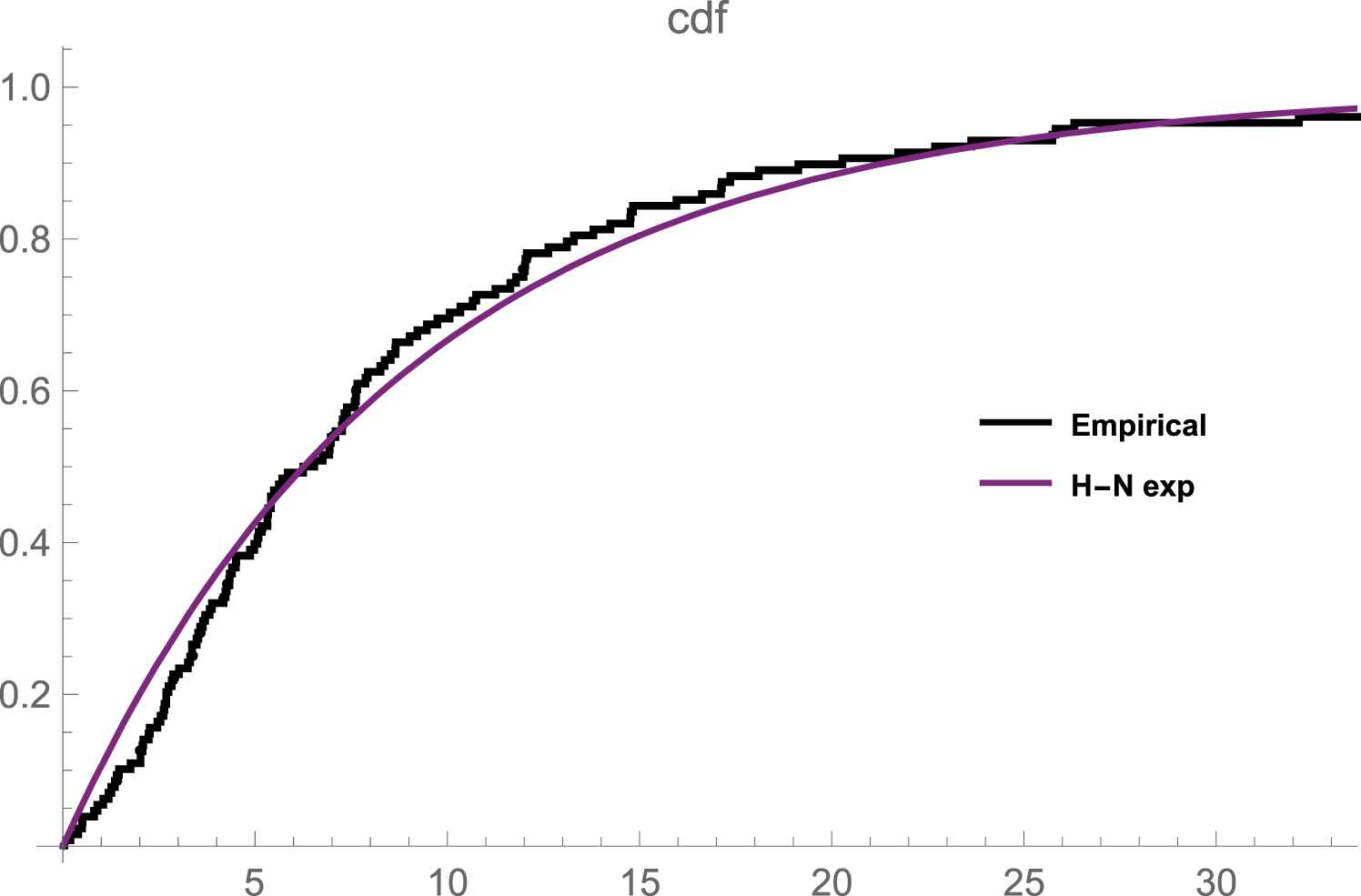
Emperical and fitted cdf plot of the remission times of bladder cancer patients data.
| n | m | Scheme | ||||
|---|---|---|---|---|---|---|
| 128 | 128 | (0 * 128)a | 0.846349 | 0.127828 | 0.873219 | 0.132073 |
| (0.648884, 1.04381) | (0.0774782, 0.178178) | |||||
| 128 | 53 | (0*53, 75) | 0.473106 | 0.244122 | 0.347462 | 0.291060 |
| (0.210417, 0.735742) | (0.0521221, 0.436122) | |||||
| 128 | 59 | (0*59, 1*69) | 1.771420 | 0.157970 | 5.94787 | 0.171523 |
| (0.99333, 2.54951) | (0.0706334, 0.245307) |
The mle (CI in parenthesis) and Bayes estimates using different censoring schemes for a This 0*3(say) denotes that 0, 0, 0.
The mle (CI in parenthesis) and Bayes estimates using different censoring schemes for the data set.
On the other hand, one can compute an approximate Bayes estimates for the two unknown parameters using the Gibbs sampling procedure which generates samples from the posterior distribution. Here, we obtain the approximate Bayes estimates under the assumptions of noninformative prior. A set of 10000 Gibbs samples was generated after a “burn-in-sample” of size 1000. Using these generated samples posterior summaries of interest can be derived and all the calculations are performed using the WinBUGS software. Table 9 lists the posterior descriptive summaries of interest. This table consists of MC error which considered as One way to assess the accuracy of the posterior estimates is by calculating the Monte Carlo error (MC error) for each parameter which estimates of the difference between the mean of sampled values and the true posterior mean. The simulation should be run until the MC error for each parameter of interest is less than about 5% of the sample standard deviation and this achieved in our example.
| n | m | Scheme | Posterior Summaries | ||
|---|---|---|---|---|---|
| 128 | 128 | (0 * 128)a | Mean (sd) | 2.856(0.1253) | 0.02215(0.001777) |
| credible interval | (2.722, 3.180) | (0.0188, 0.0256) | |||
| MC error | 0.001682 | 2.163E-5 | |||
| 128 | 53 | (0*53,75) | mean (sd) | 2.692(0.3328) | 0.04565(0.003972) |
| credible interval | (2.220, 3.454) | (0.0353, 0.04967) | |||
| MC error | 0.006645 | 7.798E-5 |
(a) This 0*3 (say) denotes that 0, 0, 0.
The approximate Bayes estimates (sd in parenthesis and credible interval under different censoring schemes for the data set.
CONFLICTS OF INTEREST
The authors declare that there is no conflict of interest.
ACKNOWLEDGMENTS
The authors are grateful to the editor and referees for their comments that helped to improve the paper.
APPENDIX
Lindley [9] developed an asymptotic expansion to evaluate the ratio of the following integral
Using Lindely's method,
The right-hand side of above equation are evaluated at the mle
Cite this article
TY  - JOUR
AU  - M. R. Mahmoud
AU  - R. M. Mandouh
PY  - 2021
DA  - 2021/03/29
TI  - Progressively Censored N-H Exponential Distribution
JO  - Journal of Statistical Theory and Applications
SP  - 267
EP  - 278
VL  - 20
IS  - 2
SN  - 2214-1766
UR  - https://doi.org/10.2991/jsta.d.210322.002
DO  - 10.2991/jsta.d.210322.002
ID  - Mahmoud2021
ER  -