
Parameter Estimation of the Weighted Generalized Inverse Weibull Distribution
- DOI
- 10.2991/jsta.d.210607.002How to use a DOI?
- Keywords
- Generalized inverse Weibull distribution; Weighted generalized inverse Weibull distribution; Loss function; Bayesian estimation
- Abstract
Weighted distributions are used widely in many fields of real life such as medicine, ecology, reliability, and so on. The idea of weighted distributions was given by Fisher and studied by Rao in a unified manner who pointed out that in many situations the recorded observations cannot be considered as a random sample from the original distribution. This can be due to nonobservability of some events, damage caused to the original observations or adoption of unequal probability sampling procedure. In this paper, we have proposed weighted version of generalized inverse Weibull distribution known as weighted generalized inverse Weibull distribution (WGIWD). Classical and Bayesian methods of estimation were proposed for estimating the parameters of the new model. The usefulness of the new model was demonstrated by applying it to a real-life data set.
- Copyright
- © 2021 The Authors. Published by Atlantis Press B.V.
- Open Access
- This is an open access article distributed under the CC BY-NC 4.0 license (http://creativecommons.org/licenses/by-nc/4.0/).
1. INTRODUCTION
In many observational studies for wild life, human, fish population or insect, every unit in the population does not have the same chance of being included in the sample. In such cases, sampling frames are not well defined and recorded observations are biased. These observations don't follow the parent distribution and hence their modeling gives birth to the theory of weighted distributions. Fisher [1] and Rao [2] introduced and unified the concept of weighted distribution. Rao identified various situations that can be modeled by weighted distributions. These situations refer to instances where the recorded observations cannot be considered as a random sample from the original distributions. This may occur due to nonobservability of some events or damage caused to the original observation, or adoption of unequal probability sampling procedure. Weighted distributions were used frequently in research related to reliability, biomedicine, ecology and branching processes can be seen in Patil and Rao [3], Gupta and Kirmani [4], Gupta and Keating [5], Oluyede [6] and in references there in. There are many researchers for weighted distribution as Das and Roy [7] discussed the length-biased weighted generalized Rayleigh distribution with its properties, Sofi et al. [8] studied the structural properties of length-biased Nakagami distribution. For more important results of weighted distribution see Oluyede and George [9], Ghitany and Al-Mutairi [10], Ahmed, Reshi and Mir [11], Sofi et al. [12].
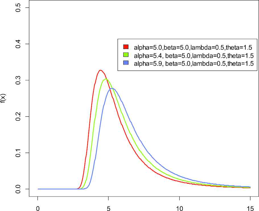
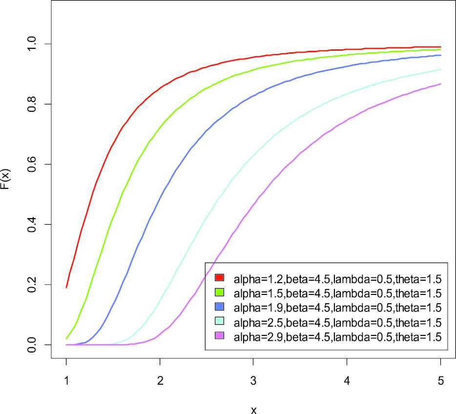
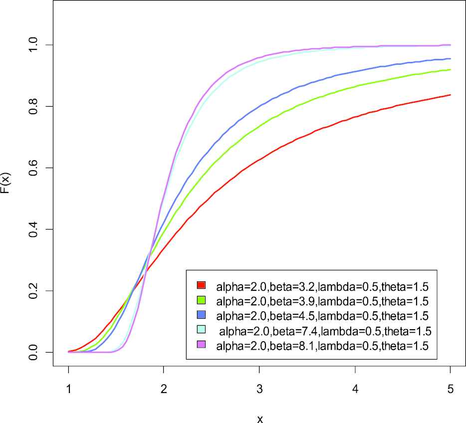
Probability distribution function of weighted generalized inverse Weibull distribution.
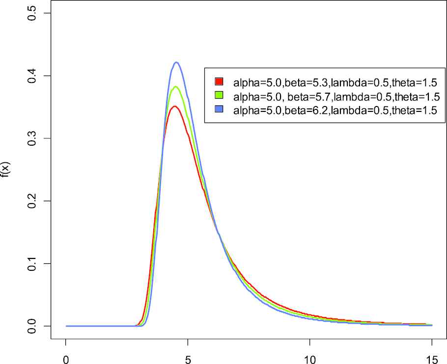
Probability distribution function of weighted generalized inverse Weibull distribution.
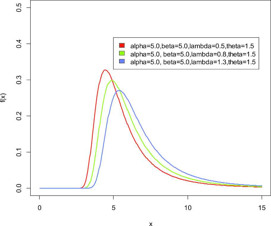
Probability distribution function of weighted generalized inverse Weibull distribution.
Suppose X is a nonnegative random variable with probability density function
The probability density function of generalized inverse Weibull distribution is given by
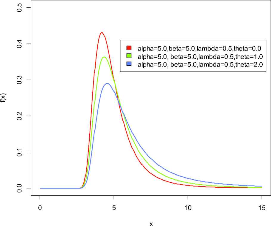
Probability distribution function of weighted generalized inverse Weibull distribution.
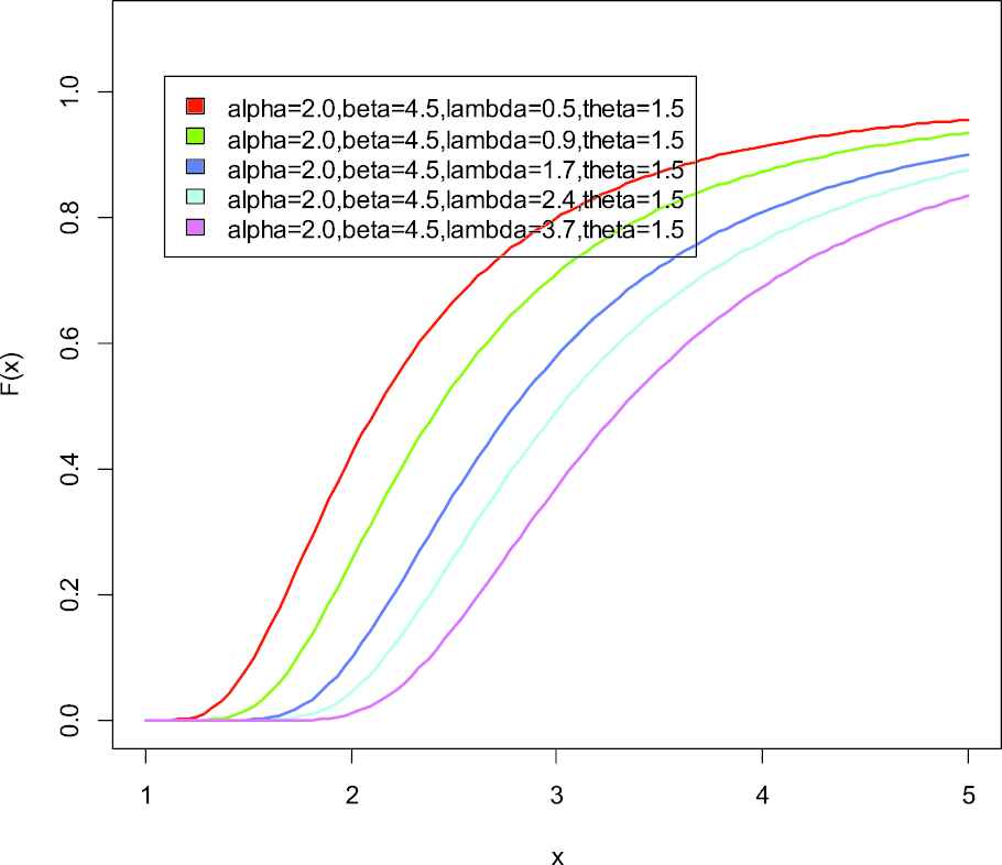
Cumulative distribution function of weighted generalized inverse Weibull distribution.
Let
Now,
Cumulative distribution function of weighted generalized inverse Weibull distribution.
Cumulative distribution function of weighted generalized inverse Weibull distribution.
Substitute the value of Equations (2)–(4) in Equation (1), we get
The density function in Equation (5) is known as weighted generalized inverse Weibull distribution (WGIWD).
Also the cumulative distribution function (cdf) of weighted generalized inverse Weibull distribution (WGIWD) is
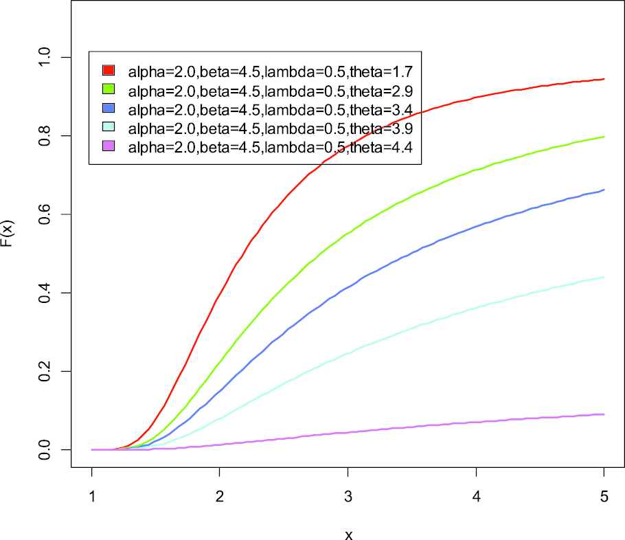
Cumulative distribution function of weighted generalized inverse Weibull distribution.
2. MAXIMUM LIKELIHOOD ESTIMATION
Let
Now differentiate the above equation with respect to α and equate to zero, we get
This is the required MLE of
3. PARAMETER ESTIMATION UNDER SQUARED ERROR LOSS FUNCTION
In this section two different prior distributions namely Jeffrey's prior and extension of Jeffrey's prior are used for estimating the scale parameter of the WGIWD.
3.1. Using Jeffrey's Prior
Consider that the parameter
Therefore, the Jeffrey's prior distribution is defined by
The posterior distribution using Jeffrey's prior is obtained by using Bayes theorem given by
With this value of
By using squared error loss function
The Bayes estimator
3.2. Using Extension of Jeffrey's Prior
The extension of Jeffrey's prior relating to the scale parameter
The posterior distribution using extension of Jeffrey's prior is obtained by using the same procedure as in case of Jeffrey's prior and is given by
By using squared error loss function
The Bayes estimator
4. PARAMETER ESTIMATION UNDER QUADRATIC LOSS FUNCTION
In this section we use quadratic loss function to obtain Bayes estimators using Jeffrey's and extension of Jeffrey's prior information.
The quadratic loss function is defined as
4.1. Using Jeffrey's Prior
By using the quadratic loss function
The Bayes estimator
4.2. Using Extension of Jeffrey's Prior
Taking the posterior distribution (11) and by using the quadratic loss function, the risk function is given by
The Bayes estimator
5. PARAMETER ESTIMATION UNDER NEW LOSS FUNCTION
In this section we obtain the Bayes estimators under new loss function introduced by Al-Bayyati [13] using Jeffrey's and extension of Jeffrey's prior
The Al-Bayyati's new loss function also called new loss function is of the form
Here we use this loss function to obtain the Bayes estimator of the scale parameter α of the WGIWD.
5.1. Using Jeffrey's Prior
By using the new loss function
The Bayes estimator
5.2. Using Extension of Jeffrey's Prior
By taking the posterior distribution (11) and using the new loss function, the risk function is given by
The Bayes estimator
6. POSTERIOR MEAN AND POSTERIOR VARIANCE OF SCALE PARAMETER UNDER JEFFREY'S AND EXTENSION OF JEFFREY'S PRIORS
In this section, we calculate the posterior mean and posterior variance of the scale parameter
6.1. Posterior Mean and Posterior Variance of Under Jeffrey's Prior
We have the posterior distribution under Jeffrey's prior as
Now
By using Equation (16) in Equation (17), we get
If r = 1 in (18), we get
This is the posterior mean
If r = 2 in (18), we get
Thus the posterior variance is given by
6.2. Posterior Mean and Posterior Variance of Under Extension of Jeffrey's Prior
We have the posterior distribution under extension of Jeffrey's prior as
Now
By using Equation (19) in Equation (20), we get
If r = 1 in (21), we get
This is the posterior mean
If r = 2 in (21), we get
Thus the posterior variance is given by
Remark 5.
If
7. DATA ANALYSIS
In this section we analyze real-life data set for illustration given by Lee and Wang [14] which represent remission times (in months) of a random sample of 128 bladder cancer patients (Table 1). A program has been developed in R language to obtain the Bayes estimates and posterior risks. The data are as follows: 0.08, 2.09, 3.48, 4.87, 6.94, 8.66, 13.11, 23.63, 0.20, 2.23, 3.52, 4.98, 6.97, 9.02, 13.29, 0.40, 2.26, 3.57, 5.06, 7.09, 9.22, 13.80, 25.74, 0.50, 2.46, 3.64, 5.09, 7.26, 9.47, 14.24, 25.82, 0.51, 2.54, 3.70, 5.17, 7.28, 9.74, 14.76, 26.31, 0.81, 2.62, 3.82, 5.32, 7.32, 10.06, 14.77, 32.15, 2.64, 3.88, 5.32, 7.39, 10.34, 14.83, 34.26, 0.90, 2.69, 4.18, 5.34, 7.59, 10.66, 15.96, 36.66, 1.05, 2.69, 4.23, 5.41, 7.62, 10.75, 16.62, 43.01, 1.19, 2.75, 4.26, 5.41, 7.63, 17.12, 46.12, 1.26, 2.83, 4.33, 5.49, 7.66, 11.25, 17.14, 79.05, 1.35, 2.87, 5.62, 7.87, 11.64, 17.36, 1.40, 3.02, 4.34, 5.71, 7.93, 11.79, 18.10, 1.46, 4.40, 5.85, 8.26, 11.98, 19.13, 1.76, 3.25, 4.50, 6.25, 8.37, 12.02, 2.02, 3.31, 4.51, 6.54, 8.53, 12.03, 20.28, 2.02, 3.36, 6.76, 12.07, 21.73, 2.07, 3.36, 6.93, 8.65, 12.63, 22.69.
| Min. | 1st Qu. | Median | Mean | 3rd Qu. | Max. | Standard deviation | Skewness | Kurtosis |
|---|---|---|---|---|---|---|---|---|
| 0.080 | 3.348 | 6.395 | 9.366 | 11.840 | 79.050 | 10.50833 | 3.286569 | 18.48308 |
Descriptive statistics for the above real data set.
By using different loss functions, that is, SELF, QLF and NLF, the Bayes estimates and posterior risk through Jeffrey's and extension of Jeffrey's priors are presented in the tables below where posterior risk are in parentheses.
8. CONCLUSION
In this paper, we have primarily estimate the scale parameter of the new model known as WGID under Jeffrey's and extension of Jeffrey's prior distributions assuming different loss functions. For comparison, we use the real-life data set and the results are shown in the tables above.
Tables 2 and 3 show the estimates and the posterior risk in parentheses of the scale parameter
| C | MLE | SELF | QLF | NLF | ||||
|---|---|---|---|---|---|---|---|---|
| 1.05 | 1.5 | 0.5 | 1 | 0.5 | 0.7981785 | 0.7971406 | 0.7887990 | 0.7992192 |
| (0.003311692) | (0.005266604) | (0.0029587057) | ||||||
| 2.0 | 0.5 | 3 | 1.0 | 0.8956767 | 0.8945112 | 0.8898279 | 0.8968437 | |
| (0.006259293) | (0.002628107) | (0.0018663487) | ||||||
| 2.5 | 1.0 | 4 | 1.5 | 0.8374464 | 0.8361384 | 0.8326298 | 0.8387554 | |
| (0.005839690) | (0.002105796) | (0.0011153567) | ||||||
| 3.5 | 1.5 | 6 | 2.0 | 0.8687908 | 0.8675784 | 0.8656269 | 0.8695190 | |
| (0.005057925) | (0.001127539) | (0.0006331024) | ||||||
| 3.97 | 1.5 | 0.5 | 1 | 0.5 | 0.3288763 | 0.3284486 | 0.3250116 | 0.3293051 |
| (0.0005622312) | (0.005266605) | (0.0003224283) | ||||||
| 2.0 | 0.5 | 3 | 1.0 | 0.4606284 | 0.4600290 | 0.4576205 | 0.4612285 | |
| (0.0016554805) | (0.002628793) | (0.0002538581) | ||||||
| 2.5 | 1.0 | 4 | 1.5 | 0.4919450 | 0.4911766 | 0.4891155 | 0.4927139 | |
| (0.0020151567) | (0.002105852) | (0.0001732894) | ||||||
| 3.5 | 1.5 | 6 | 2.0 | 0.5941366 | 0.5933075 | 0.5919729 | 0.5946346 | |
| (0.0023654540) | (0.001127542) | (0.0001384708) | ||||||
| 4.12 | 1.5 | 0.5 | 1 | 0.5 | 0.3208446 | 0.3204274 | 0.3170743 | 0.3212629 |
| (0.0005351054) | (0.005266658) | (0.0003031018) | ||||||
| 2.0 | 0.5 | 3 | 1.0 | 0.4521654 | 0.4515770 | 0.4492128 | 0.4527545 | |
| (0.0015952082) | (0.002628331) | (0.0002401214) | ||||||
| 2.5 | 1.0 | 4 | 1.5 | 0.4847009 | 0.4839439 | 0.4819132 | 0.4854585 | |
| (0.0019562459) | (0.002105828) | (0.0001645215) | ||||||
| 3.5 | 1.5 | 6 | 2.0 | 0.5878742 | 0.5870538 | 0.5857333 | 0.5883669 | |
| (0.0023158514) | (0.001127543) | (0.0001327244) |
MLE = maximum likelihood estimator, SELF = square error loss function, QLF = quadratic loss function, NLF = new loss function.
Estimates and (posterior risk) of
| C | MLE | SELF | QLF | NLF | |||||
|---|---|---|---|---|---|---|---|---|---|
| 1.05 | 1.5 | 0.5 | 1 | 0.5 | 0.5 | 0.7981785 | 0.7971406 | 0.7887990 | 0.7992192 |
| (0.003311692) | (0.005266604) | (0.0029587057) | |||||||
| 2.0 | 0.5 | 3 | 1.0 | 1.0 | 0.8956767 | 0.8921727 | 0.8874770 | 0.8945112 | |
| (0.006259250) | (0.002641994) | (0.0018614567) | |||||||
| 2.5 | 1.0 | 4 | 2.0 | 1.5 | 0.8374464 | 0.8308672 | 0.8273250 | 0.8335090 | |
| (0.005858038) | (0.002139587) | (0.0011082842) | |||||||
| 3.5 | 1.5 | 6 | 2.5 | 2.0 | 0.8687908 | 0.8636644 | 0.8616906 | 0.8656269 | |
| (0.005092232) | (0.001145624) | (0.0006316363) | |||||||
| 3.97 | 1.5 | 0.5 | 1 | 0.5 | 0.5 | 0.3288763 | 0.3284486 | 0.3250116 | 0.3293051 |
| (0.0005622312) | (0.005266605) | (0.0003224283) | |||||||
| 2.0 | 0.5 | 3 | 1.0 | 1.0 | 0.4606284 | 0.4588263 | 0.4564114 | 0.4600290 | |
| (0.0016554692) | (0.002642805) | (0.0002531927) | |||||||
| 2.5 | 1.0 | 4 | 2.0 | 1.5 | 0.4919450 | 0.4880801 | 0.4859993 | 0.4896320 | |
| (0.0020214881) | (0.002143806) | (0.0001721906) | |||||||
| 3.5 | 1.5 | 6 | 2.5 | 2.0 | 0.5941366 | 0.5906308 | 0.5892810 | 0.5919729 | |
| (0.0023814988) | (0.001145851) | (0.0001381502) | |||||||
| 4.12 | 1.5 | 0.5 | 1 | 0.5 | 0.5 | 0.3208446 | 0.3204274 | 0.3170743 | 0.3212629 |
| (0.0005351054) | (0.005266658) | (0.0003031018) | |||||||
| 2.0 | 0.5 | 3 | 1.0 | 1.0 | 0.4521654 | 0.4503964 | 0.4480259 | 0.4515770 | |
| (0.0015951972) | (0.002641997) | (0.0002394920) | |||||||
| 2.5 | 1.0 | 4 | 2.0 | 1.5 | 0.4847009 | 0.4808930 | 0.4788428 | 0.4824220 | |
| (0.0019623923) | (0.002139695) | (0.0001634783) | |||||||
| 3.5 | 1.5 | 6 | 2.5 | 2.0 | 0.5878742 | 0.5844053 | 0.5830697 | 0.5857333 | |
| (0.0023315597) | (0.001145638) | (0.0001324170) |
MLE = maximum likelihood estimator, SELF = square error loss function, QLF = quadratic loss function, NLF = new loss function.
Estimates and (posterior risk) of
CONFLICTS OF INTEREST
The authors declare they have no conflicts of interest.
AUTHORS' CONTRIBUTIONS
Authors developed the new model and performed the analytical calculations. They also discussed the results and contributed to the final manuscript.
ACKNOWLEDGMENTS
The authors are very much thankful to the reviewers for their valuable inputs to bring this research paper to this form.
REFERENCES
Cite this article
TY  - JOUR
AU  - Sofi Mudasir
AU  - S.P. Ahmad
PY  - 2021
DA  - 2021/07/10
TI  - Parameter Estimation of the Weighted Generalized Inverse Weibull Distribution
JO  - Journal of Statistical Theory and Applications
SP  - 395
EP  - 406
VL  - 20
IS  - 2
SN  - 2214-1766
UR  - https://doi.org/10.2991/jsta.d.210607.002
DO  - 10.2991/jsta.d.210607.002
ID  - Mudasir2021
ER  -