
Estimation of Parameters of the GIE Distribution Under Progressive Type-I Censoring
 , Ashraf D. Abdellatif3
- DOI
- 10.2991/jsta.d.210510.001How to use a DOI?
- Keywords
- Generalized inverted exponential distribution; Progressive Type-I censoring scheme; Maximum likelihood estimation; Bayesian estimation; Markov chain Monte Carlo; Metropolis–Hasting algorithm
- Abstract
In this paper, we consider generalized inverted exponential distribution which is capable of modeling various shapes of failure rates and aging processes. Based on progressive Type-I censored data, we consider the problem of estimation of parameters under classical and Bayesian approaches. In this regard, we obtain maximum likelihood estimates and Bayes estimates under squared error loss function. We also compute a 95% asymptotic confidence interval, bootstrap confidence intervals and highest posterior density (HPD) credible interval estimates. Finally, we analyze a real data set and conduct a Monte Carlo simulation study to compare the performance of the various proposed estimators.
- Copyright
- © 2021 The Authors. Published by Atlantis Press B.V.
- Open Access
- This is an open access article distributed under the CC BY-NC 4.0 license (http://creativecommons.org/licenses/by-nc/4.0/).
1. INTRODUCTION
Inverted distributions have been introduced to overcome some disadvantages of many widely used distributions in reliability and survival analysis. These disadvantages include constant hazard (failure) rates of an exponential distribution and nonclosed form of some distribution functions such as gamma distribution. The inverted exponential (IE) distribution has been studied and used to overcome the restriction of the constant hazard rate. Lin et al. [1] studied the properties of the IE distribution such as reliability function, hazard rate, and estimation of the parameters by using maximum likelihood method. While, Dey [2] studied the IE distribution from the Bayesian viewpoint depended on squared error and LINEX loss functions. The generalized inverted exponential (GIE) distribution has been proposed by Abouammoh and Alshingiti [3]. This lifetime distribution can be considered as another useful two-parameter generalization of the IE distribution.
The probability density function (pdf) and cumulative distribution function (cdf) of the GIE distribution are respectively given by
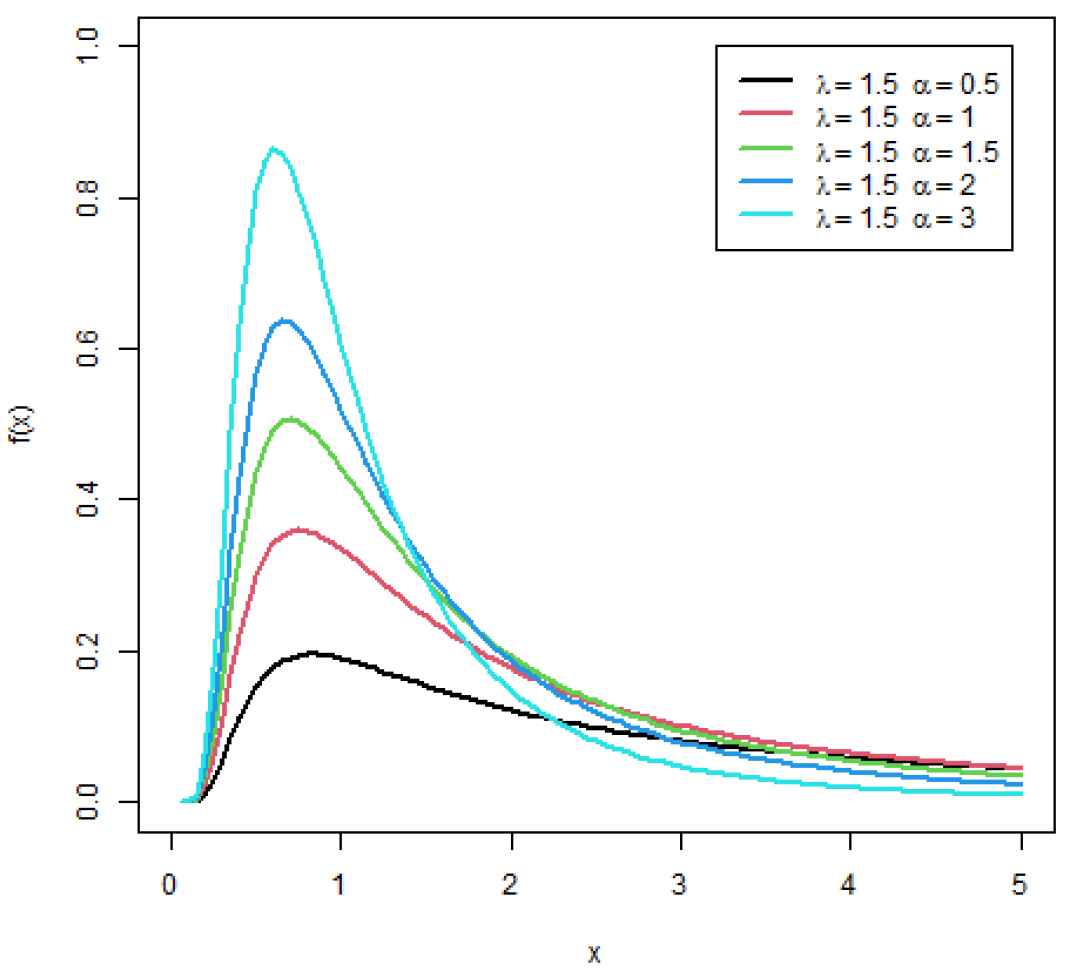
Density function of GIE distribution for some values of α.
The hazard rate function of GIE distribution can be obtained from
Abouammoh and Alshingiti [3] studied some characteristics and properties of GIE distribution in details. The hazard (failure) rate function of GIE distribution can be increasing in the beginning of the ageing and decreasing in the end of the ageing but never constant relying on the shape parameter. The GIE distribution has a right skewed density function and unimodal. Also, they investigated that the GIE distribution can provide a better fit than Weibull, generalized exponential, gamma, and IE distributions. The recent contributions of the GIE distribution are the studies made by Krishna and Kumar [4], Dey and Dey [5,6], Dey and Pradhan [7], Dey et al. [8], Singh et al. [9], Singh et al. [10], and Dube et al. [11].
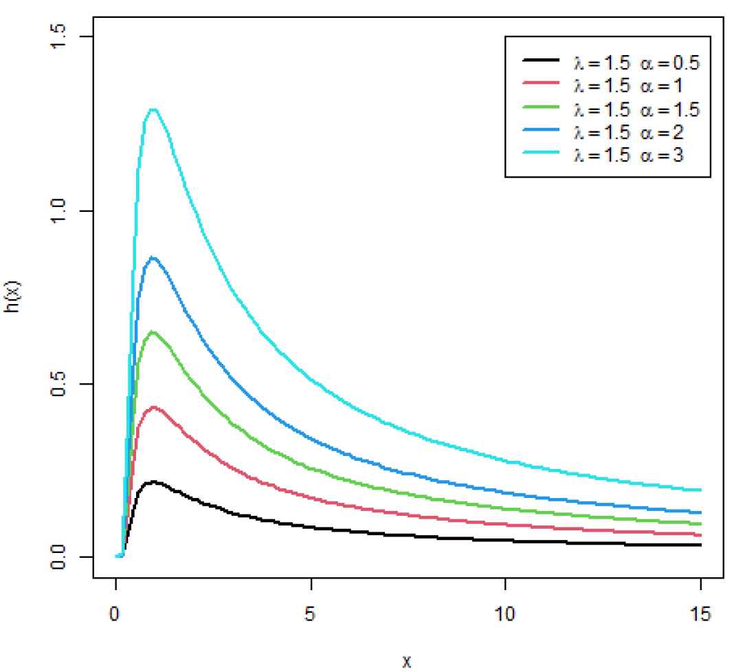
Hazard rate function of GIE distribution for some values of α.
In practical life-testing experiment, censored data arise when the experiments including the lifetimes of test units have to be terminated before collecting complete observation. The censoring technique is common and unavoidable in practice for many reasons such as time constraint and cost reduction. Various kinds of censoring have been discussed in the literature, with the most common censoring schemes being Type-I censoring and Type-II censoring. Recently, a generalized form of censoring named progressive censoring schemes has gained significant attention in the literature because of its effective utilization of the available resources in comparison with traditional censoring designs. One of these progressive censoring schemes is called progressive Type-I. This scheme occurs when a prefixed number items are removed through the experiment from the survived items at the predetermined time of censoring. It provides both the practical feature of knowing the termination time and the larger flexibility to the experimenter in the phase of design by allowing eliminating the test units at nonterminal time points. However, most of the inferential work carried out in the literature of progressive censoring have mainly focused on Type-II rather than Type-I situation. This is because progressive Type-I poses some difficulties in developing exact inference as well as in studying the theoretical properties of ordered failure times arising from such a censoring scheme while progressive Type-II PC possesses more tractable mathematical properties (Balakrishnan et al. [12]).
Suppose n units are placed on a life-testing experiment. Further, suppose X1, X2, …, Xn denote the lifetimes of these n units taken from a population with cdf F (x; θ) and pdf f(x; θ), where θ is a vector of unknown parameters of the distribution. Let x(1) < x(2) < … < x(n) denote the corresponding ordered lifetimes observed from the life test. Progressive Type-I censoring is observed when Ri items are removed from the survived items at the predetermined time of censoring Tqi corresponding to the qith quantiles, i = 1, 2, …, m, where m is the number of stages in the test, Tqi > Tqi−1 and
Based on the prior knowledge and experience of the experimenter about the items on test (Balasooriya and Low [13]), or
The quantiles of lifetimes distribution, qith, which can be determined from the following relation
F−1(.) is the inverse function from the cdf of the given distribution.
In these situations Ri; Tqi and n are fixed and predetermined while li is the number of the survivor items at time Tqi and
One can observe that complete samples and also Type-I censoring scheme can be considered as special cases of this scheme of censoring.
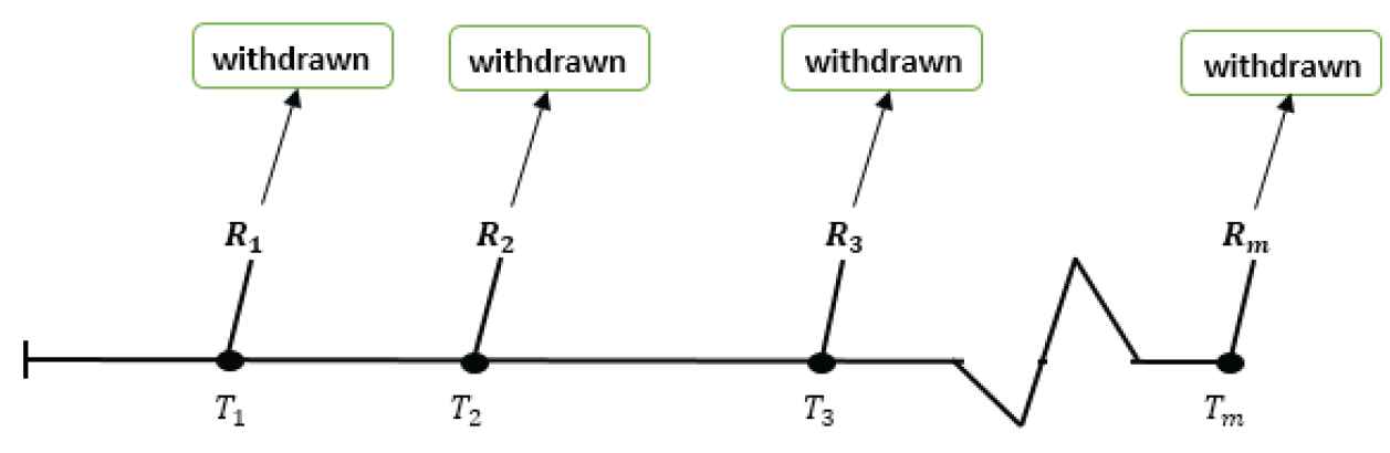
Progressive Type-I censoring scheme.
Krishna and Kumar [4] studied the GIE distribution under progressive Type-II censoring. They obtained the maximum likelihood estimator and associated asymptotic confidence intervals for the unknown parameters, and also discussed reliability characteristics and other distribution properties. Recently, Dey and Dey [6] discussed Bayes estimates and the associated highest posterior density interval estimates. They have also proved the uniqueness and existence of the maximum likelihood estimators. One may further mention to Singh et al. [16] for random removal case.
This article's goal is to investigate methods of estimation, maximum likelihood estimators (MLE), and Bayes estimators, under progressive Type-I censoring scheme. Supposing that the lifetime of the test units are independently GIE distributed, we obtained the MLEs of the unknown parameters of GIE(λ,α) distribution in Section 2. By assuming gamma prior distributions and squared error loss function, we obtained Bayes estimates using Metropolis–Hasting algorithm and the associated highest posterior density interval estimates in Section 3. Finally, a real data set is analyzed for illustrative purposes and also Monte Carlo simulations are carried out to explore the performance of the introduced estimators and comments are obtained depended on this study in Section 4.
2. MAXIMUM LIKELIHOOD ESTIMATION
In this section, we obtain MLEs for the unknown parameters of the GIE distribution based on progressive Type-I censored data. The implementation of progressive Type-I censoring scheme can be implement as follows:
Suppose that a random sample of n units whose lifetimes follows GIE(λ,α) distribution is put on a life test experiment.
Prefix m censoring time points Tq1, …, Tqm, at which fixed number R1, …, …, Rm−1 of surviving items are randomly removed from the test. The censoring times Tqi are selected corresponding to P (X ≤ Tqi) = qi, where X follows GIE(λ, α) distribution.
The life test is terminating at a pre-specified time Tqm.
Therefore, we can obtain the progressive Type-I censored samples x = (x(1), x(2), …, x(r)) that represent the observed lifetimes of the n units under this scheme of censoring. Then the associated likelihood function of λ and α given the observed data x can be written as
Taking logarithm of ℓ(λ, α) to obtain log-likelihood ln ℓ as
First partial derivatives of Log-likelihood function ln ℓ with respect to λ and α are
Equating
The numerical solution of the above two equations for
Now, one can obtain the asymptotic variance-covariance matrix of the MLEs of λ and α by inverting the negative for the expected values of second order derivatives of the log-likelihood function. That is
The approximate variance covariance matrix may be obtained by replacing expected values by their MLEs, namely; observed Fisher information matrix (Cohen, A.C. [17]). Now the approximate sample information matrix will be
2.1. Asymptotic Confidence Interval
In this sub-section, we derive the confidence intervals of the unknown parameters λ and α based on the asymptotic distribution of the MLE of the parameters. Based on the asymptotic distribution of the MLE of the parameters, it is known that
2.2. Bootstrap Confidence Intervals
In this subsection, we propose to use the two confidence intervals of the unknown parameters λ and α in presence of progressive Type-I censoring scheme based on the parametric bootstrap methods; (i) percentile bootstrap method (Boot-p CI), (ii) bootstrap-t method (Boot-t CI). There is the steps for computing the two bootstrap confidence intervals.
Boot-p CI
Generating data from GIE distribution with initial parameters λ and α and applying the progressive Type-I censoring scheme with given vector of time censoring Tqm and a vector of fixed removed items R.
Compute the MLEs of λ and α using the progressive Type-I censored data which generated in step 1.
Generate a bootstrap sample using
Repeat step (3) B times to have
Arrange
The two-sided 100(1 − γ)% Boot-p CI for the unknown parameters λ and α are given by
Boot-t CI
Same as the steps (1-3) in Boot-p CI.
Compute the t-statistic for λ and α as follows
whereRepeat step (1-2) B times to have
Arrange
The two-sided 100(1 − γ)% Boot-t CI for the unknown parameters λ and α, respectively, are given by
and
3. BAYESIAN ESTIMATION
In this section, we discuss the Bayesian estimation of the unknown parameters of the GIE distribution under progressive Type-I censoring scheme. The squared error loss function will be considered. One can suggest using independent gamma priors for both parameters of the GIE distribution λ and α having pdfs
Hyper-parameter elicitation: The elicitation of the hyper-parameters will relies on the informative priors. These informative priors will be obtained from the MLEs for (λ, α) by equating the mean and variance of
Now on solving the above two equations, the estimated hyper-parameters can be written as
The corresponding posterior density given the observed data x = (x(1), x(2), …, x(r)) can be written as
The posterior density function can be written as
Thus, the posterior density can be rewritten as
The Bayes Estimator of any function, say g(λ, α) under the squared error, is given by
Unfortunately, Eq. (8) cannot be computed for general g(λ, α).Therefore, we suggest the most common approximate Bayes estimates of λ and α Markov Chain Monte Carlo (MCMC).
MCMC is considered a computer-driven sampling technique. It permits one to characterize a distribution without knowing all of the distribution mathematical properties by random sampling values out of the distribution (Ravenzwaaij et al. [19]). MCMC is beneficial in Bayesian inference by focusing on the posterior distributions that, in most cases, are often hard to work with through analytic examination. In these cases, MCMC allows to approximate aspects of posterior distributions that cannot be directly computed (e.g., random samples from the posterior, posterior means, etc.).
Using MCMC, samples from a distribution can be drawn as follows:
Starting with an initial guess: just one value that might be plausibly drawn from the distribution.
From this initial guess, generating a series of new samples. Every new sample can be generated in two steps:
Proposal: by adding a small random perturbation to the most recent sample.
Acceptance: the new proposal is either accepted as the new sample, or rejected (in this case, the old proposal sample is retained).
There are many ways of adding random noise to generate proposals, and also diverse techniques to the process of accepting and rejecting, such as Gibbs-sampling and Metropolis–Hastings algorithm.
3.1. Metropolis–Hasting Algorithm
To perform the MH algorithm for the GIE distribution we have to define a proposal distribution and an initial values of the unknown parameters λ and α. For the proposal distribution, we consider a bivariate normal distribution, that is,
Step 1. Set initial value of
Step 2. For i = 1, 2, …, M repeat the
2.1: Set θ = θ(i−1).
2.2: Generate a new candidate parameter value δ from N2 (ln θ, Sθ.
2.3: Set θ0 = exp(δ).
2.4: Calculate
2.5: Generate a sample u from the uniform U(0, 1); distribution.
2.6: Accept or reject the new candidate θ′
Finally, from the random samples of size M drawn from the posterior density, some of the initial samples can be discarded (burn-in), and remaining samples can be further carried out to calculate Bayes estimates. More accurately the Eq. (8) can be estimated as
where lB represent the number of burn-in samples.
3.2. Highest Posterior Density
In this subsection, we utilize to construct HPD intervals for the unknown parameters λ and α of the GIE distribution under progressive Type-I censoring scheme using the samples drawn from the proposed MH algorithm in the previous subsection. Let us suppose that λ(γ) and α(γ) be the γth quantile of λ and α, respectively, that is,
Here
Now to obtain a 100(1 − γ)% HPD credible interval for λ and α, let
4. DATA ANALYSIS AND SIMULATION STUDY
The aim of this section is to set a comparison the performance of the different methods of estimation discussed in the previous sections. We analyze a real data set for illustrative purpose; also, a simulation study is employed to check the behavior of the proposed methods as well as to assess the statistical performances of the estimators under progressive Type-I censoring scheme. We used R-statistical programing language for calculation.
4.1. Real Data Analysis
The following data set represents the survival times (in days) of guinea pigs injected with different doses of tubercle bacilli. There were 72 observations listed below:
12, 15, 22, 24, 24, 32, 32, 33, 34, 38, 38, 43, 44, 48, 52, 53, 54, 54, 55, 56, 57, 58, 58, 59, 60, 60, 60, 60, 61, 62, 63, 65, 65, 67, 68, 70, 70, 72, 73, 75, 76, 76, 81, 83, 84, 85, 87, 91, 95, 96, 98, 99, 109, 110, 121, 127, 129, 131, 143, 146, 146, 175, 175, 211, 233, 258, 258, 263, 297, 341, 341, 376.
This data set was first recorded by Bjerkedal [20] and recently used to fit the inverse Weibull distribution by Kundu and Howlader [21] and to fit GIE distribution under progressive Type-II censoring scheme by Dey et al. [8].
We first check whether the GIE distribution is suitable for analyzing this data set. We report the MLEs of the parameters and the values of the negative log-likelihood criterion (NLC), Akaike's information criterion (AIC), Bayesian information criterion (BIC), and Kolmogorov–Smirnov (K–S) test statistic to judge the goodness of fit with comparison to Weibull, gamma, generalized exponential, inverse Weibull and inverse gamma distributions. The lower the values of these criteria, the better the fit. In Table 1, the parameter estimates and some goodness-of-fit statistics are obtained.
| NLC | AIC | BIC | K − S | |||
|---|---|---|---|---|---|---|
| Weibull | 110.3859 | 1.3929 | 794.3123 | 798.3128 | 802.8661 | 0.14803 |
| gamma | 47.9847 | 2.0811 | 788.5060 | 792.5100 | 797.0634 | 0.53991 |
| GExp | 58.8742 | 2.4796 | 786.2286 | 790.2327 | 794.7860 | 0.13097 |
| Inv. Weibull | 284.0959 | 1.4148 | 791.3300 | 787.2905 | 800.1841 | 0.1426 |
| Inv. Gamma | 130.1622 | 2.1657 | 785.2459 | 914.6430 | 919.1963 | 0.4253 |
| GIE | 102.5454 | 2.5390 | 783.2064 | 787.2542 | 791.8075 | 0.12031 |
Note. GExp: Generalized exponential distribution; Inv.: Inverse.
Goodness-of-fit tests for survival times of guinea pigs data set.
The reported values in Table 1 suggest that GIE distribution can be considered as an adequate model for the given data set among the compared distributions. Therefore, the given data set can be analyzed using this distribution and the MLE of
For fitting the given data set graphically, We plot the empirical cdf and the corresponding fitted cdfs for Weibull, gamma, generalized exponential, and GIE distributions, also, we plot the histogram and the corresponding fitted pdf lines for same distributions. Figure 4 showed the fitted lines for the cdfs and pdfs for the given data set and corresponding distributions. The figures also indicate that the GIE distribution provide better fit than the other distributions at least for this data set.

Estimated pdf and cdf for the given data set with corresponding distributions.
From the original data we generate four progressively Type-I censored samples with different m stages and removed items Rj at the time censoring Tqj corresponding to the selected quantiles qjth quantiles, where j = 1, 2, …, m. These different schemes can be described in Table 2.
| Scheme | m | qj(%) | Censoring time Tqj | Removed items Ri |
|---|---|---|---|---|
| I | 3 | (10, 30, 60) | (33, 58, 82) | (5, 5, Rm) |
| II | 4 | (10, 20, 40, 60) | (33, 52, 61, 82) | (5, 5, 5, Rm) |
| III | 5 | (10, 20, 30, 40, 60) | (33, 52, 58, 61, 82) | (5, 5, 5, 5, Rm) |
| IV | 5 | (0, 0, 0, 0, 60) | (0, 0, 0, 0, 82) | (0, 0, 0, 0, n − r) |
Different schemes for progressively Type-I censored samples.
Note that
In Table 3, we calculate the MLEs of the parameters λ and α and their associated 95% asymptotic confidence interval estimates and also bootstrap confidence intervals estimates (Boot.p and Boot.t). We also compute Bayes estimates utilizing the MH algorithm under the informative prior. Note that the informative prior require to generate 1000 complete samples each of size 60 from GIE(3.42, 2.54) distribution as past samples, and subsequently get the hyper parameter values as a1 = 51.32, b1 = 14.52, a2 = 19.33, b2 = 7.11. It is indicated that, while generating samples from the posterior distribution utilizing the MH algorithm, initial values of (λ, α) are considered as
However, for computational convenience, we transformed the original data by divide it on 30. In Table 3, for the given real data set, all the estimated values of MLEs and associated interval estimates (Asymptotic CI, Boot.p CI and Boot.t CI), standard errors and AILs are presented. Also, Bayesian estimation using MCMC by applying MH algorithm and associated HPD intervals, standard errors, and AILs are computed. From Table 3, it is noticed that informative Bayes estimates compete well with MLEs. The convergence of MCMC estimation for λ and α can be showed in Figure 5 in case of complete censoring.
| Sch. | Parm. | Maximum Likelihood Estimation |
Bayesian Estimation |
||||
|---|---|---|---|---|---|---|---|
| MLE St.E | Asy CI AIL | Boot.p CI AIL | Boot.t CI AIL | MH St.E | HPD CI AIL | ||
| I | λ | 3.260 0.575 | (2.225, 4.481) 2.256 | (2.136, 5.399) 3.263 | (1.827, 4.888) 3.061 | 2.948 0.560 | (1.923, 4.082) 2.159 |
| α | 2.322 0.777 | (1.211, 4.520) 3.309 | (1.313, 6.125) 4.812 | (1.176, 4.391) 3.215 | 1.982 0.699 | (0.879, 3.435) 2.556 | |
| II | λ | 3.374 0.598 | (2.298, 4.643) 2.345 | (2.173, 5.879) 3.706 | (1.779, 5.110) 3.331 | 3.040 0.566 | (1.988, 4.183) 2.194 |
| α | 2.474 0.859 | (1.263, 4.945) 3.682 | (1.328, 7.424) 6.096 | (1.186, 4.984) 3.798 | 2.084 0.734 | (0.856, 3.492) 2.636 | |
| III | λ | 3.335 0.607 | (2.245, 4.627) 2.382 | (2.141, 6.049) 3.908 | (1.630, 5.062) 3.432 | 2.990 0.589 | (1.819, 4.136) 2.317 |
| α | 2.366 0.848 | (1.182, 4.839) 3.657 | (1.265, 8.096) 6.831 | (1.085, 4.789) 3.704 | 2.012 0.756 | (0.699, 3.470) 2.771 | |
| IV | λ | 3.404 0.578 | (2.362, 4.628) 2.266 | (2.243, 5.935) 3.692 | (1.781, 5.082) 3.301 | 3.130 0.544 | (2.056, 4.178) 2.122 |
| α | 2.522 0.804 | (1.360, 4.769) 3.409 | (1.442, 7.430) 5.987 | (1.227, 4.745) 3.518 | 2.219 0.707 | (1.004, 3.542) 2.538 | |
| Complete | λ | 3.424 0.438 | (2.611, 4.326) 1.715 | (2.540, 4.713) 2.173 | (2.378, 4.537) 2.159 | 3.270 0.425 | (2.488, 4.100) 1.612 |
| α | 2.544 0.483 | (1.741, 3.670) 1.929 | (1.824, 4.061) 2.237 | (1.666, 3.610) 1.944 | 2.380 0.461 | (1.555, 3.320) 1.765 | |
Note. Sch.: Scheme; Parm.: Parameter; St.E: Standard error; Asy: Asymptotic.
Maximum likelihood, Bayesian, and associated interval estimates, standard errors, and AILs for real data set.
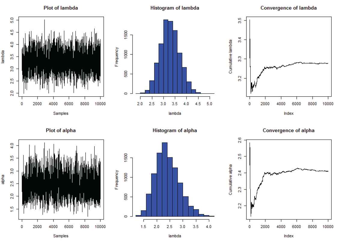
Convergence of MCMC estimates for λ and α using MH algorithm.
4.2. Simulation Study
In this subsection, we employ a Monte Carlo simulation study to compare the performance of methods of estimation; namely MLE and Bayesian estimation, under progressive Type-I censoring scheme. For the MLEs, we generate 1000 data from GIE distribution with the following assumptions:
λ = 1.5 and α = 2, i.e. GIE(1.5, 2).
Sample sizes are n = 25 and n = 100.
Number of resampling for bootstrap CI is 10000.
Number of stages of progressive Type-I censoring are m = 3, 5.
Censoring time Tqj determine corresponding to the selected
When m=3 thus qj = (10%, 30%, 60%),
When m=5 thus qj = (10%, 20%, 30%, 40%, 60%), where j = 1, 2, …, m.
Removed items Rj are proposed as
Scheme I: R1 = R2 = … = Rm−1 = 0,
Scheme II: R1 = 10, R2 = … = Rm−1 = 0,
Scheme III: R1 = R2 = … = Rm−2 = 0, Rm−1 = 10 and
Scheme IV: R1 = R2 = … = Rm−1 = 5.
where
Based on the generated data, we calculate MLEs and associated 95% asymptotic confidence interval and bootstrap confidence interval (Boot.p and Boot.t). Note that the initial guess values are considered to be same as the true parameter values while obtaining MLEs.
For Bayesian estimation method, we calculate Bayes estimates using the MH algorithm under the noninformative prior (P-I) and the informative prior (P-II). Thus
For noninformative prior (P-I), we assume that hyper-parameter values are a1 = b1 = a2 = b2 = 0, thus π(λ, α) = 1/(λα).
For informative priors (P-II), we generate 1000 complete samples each of size 60 from GIE(1.5, 2) distribution as past samples, and subsequently get the hyper parameter values as a1 = 22.74, b1 = 14.20, a2 = 9.65, b2 = 4.29.
The above values of priors (informative or non-informative) are plugged-in to calculate the desired estimates. While utilizing MH algorithm, we take into account the MLEs as initial guess values, and the associated variance–covariance matrix Sθ of
All the average estimates for both methods are reported in Tables 4 and 5. Further, the first row represents the average estimates and interval estimates, and in the second row, associated means square errors (MSEs) and average interval lengths (AILs) with coverage probabilities (CPs) are reported.
| Sch. | Parm. | MLE |
Bayesian: P-I |
Bayesian: P-II |
|||||
|---|---|---|---|---|---|---|---|---|---|
| Avg MSE | Asy CI AIL/CP | Boot.p CI AIL/CP | Boot.t CI AIL/CP | Avg MSE | HPD AIL/CP | Avg MSE | HPD AIL/CP | ||
| n = 25 | |||||||||
| I | λ | 1.659 0.341 | (0.753, 2.565) 1.812/94.80 | (1.110, 2.940) 1.830/98.40 | (0.892, 2.471) 1.579/93.40 | 1.261 0.453 | (0.200, 2.495) 2.295/96.20 | 1.511 0.067 | (0.984, 1.981) 0.997/96.40 |
| α | 2.684 5.123 | (0.185, 5.553) 5.368/95.40 | (1.639, 8.098) 6.459/98.60 | (1.401, 4.893) 3.492/92 | 1.795 2.801 | (9e-15, 4.810) 4.810/95.20 | 2.067 0.363 | (0.891, 3.161) 2.270/95.60 | |
| II | λ | 1.628 0.249 | (0.657, 2.599) 1.942/95.80 | (1.081, 3.094) 2.013/99 | (0.836, 2.437) 1.601/93.60 | 1.124 3.347 | (1e-29, 2.225) 2.225/95.20 | 1.515 0.072 | (1.077, 2.049) 0.972/97.20 |
| α | 2.713 3.912 | (0.630, 6.045) 5.415/95.20 | (1.602, 9.325) 7.723/99.20 | (1.334, 4.986) 3.652/91.60 | 6.594 4.616 | (5e-27, 5.032) 5.032/95.20 | 2.059 0.386 | (0.976, 3.266) 2.290/95.80 | |
| III | λ | 1.645 0.241 | (0.658, 2.632) 1.974/96.70 | (1.082, 2.935) 1.853/98.90 | (0.836, 2.465) 1.629/94.20 | 1.090 0.484 | (0.111, 2.181) 2.069/96.70 | 1.506 0.064 | (1.055, 2.015) 0.959/97.40 |
| α | 2.759 4.048 | (0.787, 6.305) 5.518/95.30 | (1.517, 9.623) 8.106/99.30 | (1.261, 5.533) 4.272/91.60 | 0.512 4.145 | (2e-17, 4.021) 4.021/95.30 | 2.052 0.361 | (0.911, 3.034) 2.122/95.60 | |
| IV | λ | 1.679 0.300 | (0.679, 2.679) 2.000/95.40 | (1.121, 3.010) 1.889/97.80 | (0.884, 2.487) 1.603/92.80 | 1.092 0.584 | (5e-44, 2.380) 2.380/95.20 | 1.528 0.068 | (1.059, 2.050) 0.991/97.80 |
| α | 2.931 7.180 | (0.821, 6.693) 5.672/95.40 | (1.650, 9.321) 7.671/98 | (1.372, 5.814) 4.442/92.60 | 4.152 7.962 | (9e-31, 5.592) 5.592/95.20 | 2.031 0.349 | (0.954, 3.164) 2.211/96.60 | |
| n = 100 | |||||||||
| I | λ | 1.539 0.045 | (1.114, 1.964) 0.850/96.40 | (1.197, 2.032) 0.835/98.20 | (1.150, 1.966) 0.815/96.40 | 1.451 0.093 | (0.863, 2.026) 1.163/96.40 | 1.522 0.038 | (1.149, 1.882) 0.733/97.20 |
| α | 2.152 0.305 | (1.114, 3.190) 2.076/94.60 | (1.596, 3.236) 1.640/95.40 | (1.513, 2.977) 1.464/92.20 | 1.971 0.497 | (0.812, 3.376) 2.564/95.80 | 2.086 0.228 | (1.187, 2.974) 1.787/96.40 | |
| II | λ | 1.538 0.052 | (1.103, 1.972) 0.869/95.80 | (1.193, 2.044) 0.851/97 | (1.142, 1.969) 0.826/95.60 | 1.441 0.102 | (0.880, 2.064) 1.184/96.80 | 1.502 0.037 | (1.167, 1.864) 0.697/98.20 |
| α | 2.129 0.367 | (1.053, 3.206) 2.152/94 | (1.564, 3.258) 1.694/95 | (1.474, 2.974) 1.500/91.80 | 1.934 0.577 | (0.823, 3.357) 2.534/96 | 2.004 0.222 | (1.094, 2.877) 1.783/96.20 | |
| III | λ | 1.551 0.054 | (1.114, 1.988) 0.874/96.40 | (1.204, 2.055) 0.851/96.80 | (1.153, 1.983) 0.830/96.40 | 1.457 0.093 | (0.891, 2.027) 1.136/96.40 | 1.517 0.038 | (1.123, 1.871) 0.748/96 |
| α | 2.168 0.376 | (1.065, 3.271) 2.206/96.40 | (1.582, 3.331) 1.749/96.40 | (1.495, 3.051) 1.556/92.60 | 1.969 0.545 | (0.741, 3.413) 2.672/95.80 | 2.061 0.225 | (1.200, 3.000) 1.800/96.80 | |
| IV | λ | 1.534 0.055 | (1.101, 1.968) 0.867/95.60 | (1.188, 2.037) 0.849/97.40 | (1.140, 1.968) 0.828/95.60 | 1.438 0.096 | (0.913, 2.024) 1.111/96 | 1.518 0.041 | (1.125, 1.905) 0.780/96.80 |
| α | 2.124 0.357 | (1.047, 3.200) 2.153/95.40 | (1.550, 3.254) 1.704/95.60 | (1.469, 2.989) 1.520/91.20 | 1.955 0.585 | (0.846, 3.478) 2.632/95.80 | 2.065 0.237 | (1.242, 3.054) 1.812/97.60 | |
Note. Sch.: Scheme; Parm.: Parameter; Avg: average; Asy CI: asymptotic confidence interval.
Average estimated values, interval estimates, MSEs, AILs, and CPs (in %) of GIE distribution with λ = 1.5 and α = 2 under m = 3.
| Sch. | Parm. | MLE |
Bayesian: P-I |
Bayesian: P-II |
|||||
|---|---|---|---|---|---|---|---|---|---|
| Avg MSE | Asy CI AIL/CP | Boot.p CI AIL/CP | Boot.t CI AIL/CP | Avg MSE | HPD AIL/CP | Avg MSE | HPD AIL/CP | ||
| n = 25 | |||||||||
| I | λ | 1.635 0.246 | (0.736, 2.535) 1.799/94.60 | (1.092, 2.913) 1.821/97.80 | (0.873, 2.438) 1.565/93.60 | 1.242 0.402 | (1.051, 2.266) 1.215/95.2 | 1.529 0.0720 | (1.021, 2.089) 1.068/97.60 |
| α | 2.500 2.1265 | (0.049, 5.049) 5.000/94.00 | (1.554, 7.764) 6.210/99.20 | (1.325, 4.405) 3.080/90.20 | 1.685 1.954 | (0.178, 4.654) 4.475/95.80 | 2.046 0.355 | (1.017, 3.277) 2.260/96.60 | |
| II | λ | 1.635 0.283 | (0.654, 2.617) 1.963/96 | (1.082, 3.136) 2.054/99 | (0.831, 2.453) 1.622/93 | 1.061 0.574 | (0.988, 2.168) 1.180/95.20 | 1.523 0.074 | (1.014, 2.073) 1.059/97 |
| α | 2.710 4.386 | (0.672, 6.093) 5.421/95.40 | (1.584, 10.793) 9.209/99 | (1.312, 5.047) 3.735/90 | 1.656 5.302 | (0.212, 4.273) 4.061/95.2 | 2.0417 0.3971 | (0.954, 3.333) 2.379/96.60 | |
| III | λ | NA | NA | NA | NA | NA | NA | NA | NA |
| α | NA | NA | NA | NA | NA | NA | NA | NA | |
| IV | λ | NA | NA | NA | NA | NA | NA | NA | NA |
| α | NA | NA | NA | NA | NA | NA | NA | NA | |
| n = 100 | |||||||||
| I | λ | 1.534 0.051 | (1.108, 1.961) 0.853/96.20 | (1.196, 2.029) 0.833/97.40 | (1.145, 1.957) 0.812/95.80 | 1.458 0.091 | (0.902, 2.019) 1.117/96.60 | 1.515 0.043 | (1.130, 1.940) 0.810/98 |
| α | 2.116 0.316 | (1.090, 3.141) 2.051/96 | (1.571, 3.183) 1.612/96.20 | (1.487, 2.925) 1.438/92.20 | 1.942 0.478 | (0.860, 3.367) 2.507/96 | 2.067 0.231 | (1.198, 3.018) 1.820/97 | |
| II | λ | 1.536 0.047 | (1.105, 1.968) 0.863/96.40 | (1.195, 2.042) 0.847/98.40 | (1.141, 1.963) 0.822/96.40 | 1.441 0.087 | (0.879, 1.976) 1.097/96.20 | 1.511 0.042 | (1.149, 1.932) 0.783/98 |
| α | 2.155 0.345 | (1.072, 3.237) 2.165/96 | (1.588, 3.291) 1.703/96.80 | (1.494, 2.999) 1.505/92 | 1.951 0.518 | (0.766, 3.325) 2.559/95.60 | 2.074 0.240 | (1.204, 3.005) 1.801/96.20 | |
| III | λ | 1.534 0.053 | (1.100, 1.968) 0.868/95.80 | (1.188, 2.036) 0.848/97 | (1.138, 1.967) 0.829/95.80 | 1.453 0.099 | (0.845, 2.046) 1.201/96.20 | 1.509 0.040 | (1.138, 1.914) 0.776/97.20 |
| α | 2.128 0.336 | (1.053, 3.204) 2.151/95.20 | (1.554, 3.278) 1.724/96 | (1.469, 3.000) 1.531/93 | 1.954 0.576 | (0.733, 3.563) 2.830/95.80 | 2.042 0.212 | (1.299, 2.961) 1.662/98 | |
| IV | λ | 1.536 0.057 | (1.094, 1.979) 0.885/96.80 | (1.187, 2.048) 0.861/98.20 | (1.133, 1.972) 0.839/96.80 | 1.442 0.101 | (0.841, 2.024) 1.183/96.40 | 1.508 0.042 | (1.099, 1.910) 0.811/97.60 |
| α | 2.151 0.408 | (1.006, 3.295) 2.289/95 | (1.548, 3.366) 1.818/95.80 | (1.457, 3.068) 1.611/93.40 | 1.944 0.652 | (0.761, 3.612) 2.851/95.80 | 2.032 0.245 | (1.101, 2.983) 1.882/96.20 | |
Note. Sch.: Scheme; Parm.: Parameter; Avg: average; Asy CI: asymptotic confidence interval.
Average estimated values, interval estimates, MSEs, AILs, and CPs (in %) of GIE distribution with λ = 1.5 and α = 2 under m = 5.
From tabulated values it can be noticed that depended on MSEs, higher values of n lead to better estimates. It is also noticed that the maximum likelihood estimates compete well with non-informative Bayes estimates, and the performance of the Bayes estimates obtained under informative prior is better than the noninformative Bayes estimates. It can also be noticed that under informative prior the AILs and associated CPs of HPD intervals are better than those of noninformative priors. Furthermore, it is also seen that, in scheme II and scheme III, MSEs, and AILs of associated interval estimates are generally lower when the units are removed at early stages.
5. CONCLUSION
In this paper, we have studied the problem of estimation and prediction for generalized IEl distribution under progressive Type-I censoring from classical and Bayesian viewpoints. We derived maximum likelihood estimates and associated asymptotic and parametric bootstrap confidence intervals estimates for the unknown parameters of the GIE distribution. Then, we calculated Bayes estimates and the corresponding HPD interval estimates under non-informative and informative priors. Also, a discussion of how to select the values of hyper-parameters in Bayesian estimation is investigated based on past samples when informative prior is taken into consideration. The simulation results indicates that MLEs is better than the noninformative Bayes estimates, and the performance of estimates under informative prior is better than both the noninformative prior and MLEs. For future work, we have considered Bayesian estimation under the squared error loss function, other loss functions can also be considered. Also, the present work can be extended to design of optimal progressive censoring sampling plan and other censoring schemes can also be considered.
CONFLICTS OF INTEREST
There is no conflict of interest in this artide.
AUTHORS' CONTRIBUTIONS
First two authors wrote the initial draft of the paper and supervised overall work. The last two authors did the analysis and analyzing the results of real data and simulation part.
Funding Statement
We have solely funded the research by ourself.
ACKNOWLEDGMENTS
The authors thank the anonymous referee for a careful reading of the article.
REFERENCES
Cite this article
TY  - JOUR
AU  - Mahmoud R. Mahmoud
AU  - Hiba Z. Muhammed
AU  - Ahmed R. El-Saeed
AU  - Ashraf D. Abdellatif
PY  - 2021
DA  - 2021/05/19
TI  - Estimation of Parameters of the GIE Distribution Under Progressive Type-I Censoring
JO  - Journal of Statistical Theory and Applications
SP  - 380
EP  - 394
VL  - 20
IS  - 2
SN  - 2214-1766
UR  - https://doi.org/10.2991/jsta.d.210510.001
DO  - 10.2991/jsta.d.210510.001
ID  - Mahmoud2021
ER  -