
Inference in Simple Step-Stress Accelerated Life Tests for Type-II Censoring Lomax Data

- DOI
- 10.2991/jsta.d.210406.001How to use a DOI?
- Keywords
- Confidence and prediction intervals; Conditional median predictor; Cumulative exposure model; Highest conditional density; Lomax distribution; Maximum likelihood estimation; Maximum likelihood prediction; Pivot quantity; Step-stress accelerated life test
- Abstract
In this paper, step-stress accelerated life test is considered to obtain the failure time data of highly reliable units in specified conditions. It is assumed that the lifetime data of such units follow Lomax distribution with a scale parameter depends on the stress level and the shape parameter remains constant. It is also assumed that failure times occur according to a cumulative exposure model (CEM). Using this model, the maximum likelihood estimators (MLEs) and the respective confidence intervals (CIs) based on the asymptotic normality theory as well as the ones based on parametric bootstrap method are considered. In the context of prediction, point and interval predictions are also addressed. A simulation study has been performed to assess the estimation and prediction methods and a real dataset is analyzed for illustrative purposes.
- Copyright
- © 2021 The Authors. Published by Atlantis Press B.V.
- Open Access
- This is an open access article distributed under the CC BY-NC 4.0 license (http://creativecommons.org/licenses/by-nc/4.0/).
1. INTRODUCTION
Accelerated Life Tests (ALT) are commonly used to evaluate the lifetime of highly reliable products or components within a reasonable testing time. In ALT the products or components are run at higher than usual levels of stress (including temperature, voltage, pressure, etc.) to obtain failures quickly. The data obtained from such an accelerated test are then transformed to estimate the distribution of failures under specified conditions. The model of ALT is chosen according to the relationship between the parameters of the failure distribution and accelerated stress conditions. If a constant stress level is used and some selected stress levels are very low, there are many nonfailed products or components during the testing time, which reduces the effectiveness of accelerated tests. To overcome this problem, step-stress accelerated life test (SSALT) are used. Detailed discussions on ALT tests can be found in Nelson [1], Lawless [2], Kundu and Ganguly [3].
In the SSALT, the stress level in the model will be changed in steps at various intermediate stages of experiment. Specifically, a test unit is subjected to a specified level of stress for a prefixed period of time, if it does not fail during that period of time, then the stress level is increased for future prefixed time. This process continues until the test units fail or some termination conditions are met. The SSALT with two levels of stress is known as simple SSALT. Miller and Nelson [4] described an optimal simple step-stress plan for (ALT) when failure times are exponentially distributed and not censored. Bai et al. [5] extended the results of Miller and Nelson [4] to the case of censoring. Bai and Kim [6] presented an optimum simple step-stress testing for the Weibull distribution under Type I censoring. Xiong [7] assumed that the mean life of an experimental unit is a log-linear function of the stress level. Based on this assumption, he developed inference for the parameters of the log-linear link function.
The censoring data is of natural interest in survival, reliabilityand medical studies due to cost or time considerations. The Type-II censoring scheme is one of the popular mechanisms of collecting data in lifetime analysis. It is often used in testing of equipment where all items are put on test at the same time and the test is terminated when the predetermined r number of the items have failed. Balakrishnan et al. [8] presented point and interval estimation for a simple step-stress model with Type-II censoring for exponential distribution. Kateri and Balakrishnan [9] estimated the original parameters of a simple step-stress model for the Weibull distribution under Type-II censoring. Watkins [10] argued that it is preferable to work with the original parameters in step-stress model, see also Kundu and Ganguly [3].
For Pareto distribution, Kamal et al. [11] presented estimates of the parameters for simple step-stress model of Pareto distribution for uncensored data. Chandra and Khan [12] considered the simple step-stress model, and obtained estimators of the parameters for Lomax with Type-I censoring. Hassan et al. [13] considered the SSALTs based on an adaptive Type-II progressive hybrid censoring with product's lifetime following Lomax distribution where the scale parameter of the lifetime distribution at any stress level is assumed to be log-linear function of the stress level.
The prediction of future censored observations based on the information available is a fundamental problem in statistics. It is widely used in survival, medical and engineering studies. For detailed discussions on point and interval prediction, one may refer to Kaminsky and Rhodin [14], Asgharzadeh et al. [15] and Saadati Nik et al. [16]. In the context of ALT, Basak and Balakrishnan [17,18] considered the problem of predicting the failure times of censored items for a simple step-stress model from exponential distribution with progressive Type-II censoring and Type-II right censoring, respectively.
The main aim of this paper is to estimate the original parameters of the model and then predict future order statistics based on Type-II censored Lomax data under simple step-stress with cumulative exposure model (CEM). It may worth mentioning that no attention has been paid for the problem of prediction of future lifetimes of Lomax distribution under CEM. Details of the model are given in Section 2. Based on the proposed model, maximum likelihood estimation procedure and its asymptotic normality are discussed in Section 3. Confidence intervals (CIs) based on the asymptotic normality of the maximum likelihood estimators (MLEs) and bootstrap methods are established in Section 4. We tackle the problem of predicting the future failure times in Section 5. A simulation study for assessing the estimation and prediction methods discussed in the previous sections are performed in Section 6. Finally, the paper is concluded in Section 7.
2. MODEL DESCRIPTION AND RELATED ASSUMPTIONS
Here, we give a description of the Lomax CEM for simple step-stress model, terminologies and its related assumptions.
Notations:
Basic assumptions:
Units are tested at two stress levels
The failure times of the units for any stress level follow Lomax distribution;
The scale parameters for the life distribution are
Failures follow the CEM.
In step-stress model, a CEM is assumed in which the lifetime distribution of the units at one stress level is related to the lifetime distribution of the units at the next level. The model assumes that the remaining lifetime of the experiment units depends only the cumulative exposure the units have experienced, with no memory on how this exposure was accumulated, see Kundu and Ganguly [3].
Lomax distribution, is a special case of the second kind of Pareto distribution, it was proposed by Lomax [19]. It has been shifted from Pareto distribution so that its support begins at zero. It has been used in business, economics, insurance, queueing theory and engineering. Its pdf is given by
So Lomax distribution may describe the lifetime of a decreasing failure rate items. Bryson [20] recommended Lomax distribution as an alternative to the exponential distribution when the data are heavy tailed.
The test is conducted as follows. All
The CEM for simple step-stress test is given by
As a consequence of that, the Lomax CEM for simple step-stress model is:
3. MAXIMUM LIKELIHOOD ESTIMATION
In this section, we consider the MLEs of the parameters
The likelihood function based on the censored data,
From the likelihood function given in (7a), (7b) and (7c), it is observed that the MLEs of the parameters exist only if
Using (5) and (6), we immediately have
Consequently, the log-likelihood function
So, the likelihood equations are given by
From (13), The MLE
The estimation procedure, through Eqs. (11)–(13), does not result in closed form. Therefore, Eqs. (11) and (12) can be solved numerically using Newton–Raphson method and the resulting estimates are denoted by
4. CIs FOR THE MODEL PARAMETERS
Here, we present two different methods for constructing CIs for the unknown parameters
4.1. Approximate CIs
It is known that for large sample sizes and under some regularity conditions, the MLEs are consistent and normally distributed
Let
So, the observed FI matrix is given by
The inverse of FI is the asymptotic variance-covariance matrix of the MLEs
So, the
4.2. Bootstrap CIs
The parametric bootstrap sampling is used to construct CIs for the unknown parameters
Algorithm for computing bootstrap CIs:
Step 1: Compute the MLEs of
Step 2: Simulate the first r order statistics
Step 3: For given value of stress change time
Step 4: The ordered observations
Step 5: Compute the MLEs of
Step 6: Repeat steps 2–5
5. PREDICTION OF FUTURE ORDER STATISTICS
In this section, we consider the problem of prediction of future failure time based on some observed failure times under the current simple step-stress model. The problem can be expressed as follows. Let
Using the Markovian property of censored order statistics, it is well-known that the conditional distribution of
5.1. Point Prediction
In this subsection, we present two techniques for obtaining point predictors of future lifetimes,
5.1.1. Maximum likelihood predictor (MLP)
The MLP was proposed by Kaminsky and Rhodin [14]. This method involves prediction of future order statistics and also estimation of the parameters in the model. The predictive likelihood function (PLF) of
Considering the case when
Consequently, the log PLF can be written as
By (34), the predictive likelihood equations (PLEs) for
Since Eqs. (35)–(38) cannot be solved analytically, numerical methods will be used to solve them simultaneously, which leads to find the MLP of
5.1.2. Conditional median predictor (CMP)
The CMP was first suggested by Raqab and Nagaraja [21]. A predictor
Based on the conditional distribution of
It can be shown that, given
5.2. Prediction Intervals (PIs)
Another aspect of prediction problem is to predict the future unobserved order statistics by constructing PIs for
5.2.1. Pivotal-based PIs
Let us consider the random variable
It can be easily shown that the conditional density in (30) is a unimodal function of
Since
5.2.2. Highest conditional density PIs
Now we consider the conditional distribution of
The density in (44) is unimodal function. An interval
Eqs. (45) and (46) can be simplified as
For the special case when
When
Finally, when
So, a
6. SIMULATION STUDY AND DATA ANALYSIS
Here in this section, we conduct a simulation study to compute the MLEs of the parameters under the simple step-stress model, as well the corresponding CIs. Computations of the prediction methods are described in another simulation experiment. A real dataset is considered to illustrate the different techniques proposed in this paper.
6.1. Simulation Study
In this section, we perform an intensive Monte Carlo (MC) simulation study for computing the MLEs
Algorithm for generating the data and finding the MLEs:
Step 1: Generate a random sample of size
Step 2: Find the random variable
Step 3: Generate a sample based on observed failure times data as follows:
Step 4: Compute the MLEs of
Also, the CIs of the parameters and PIs of the censored lifetimes are computed. The simulation process is repeated
The respective expressions for prediction bias and mean square prediction error (MSPE) can be also defined. The respective ACIs and BCIs are obtained using Eqs. (24–29) and the PIs of
The MLEs of
It is clear that the MSEs and biases of the estimates decrease as
As
It can be noticed from the values presented in the tables that the MSEs of
For the interval estimation, it is easily checked that the CIs obtained by bootstrap method outperform the ones based on the asymptotic normality approach. As a result of that, BCIs of
For prediction problem, we notice that the prediction biases of the CMP are smaller than those of the MLP for all the considered cases. By considering the MSPE as an optimality criterion, it is checked that, the CMP performs better than the MLP. However, the ratio of MSPEs of MLPs to the MSPEs of CMPs becomes closer to 1 in many cases, especially when
As expected, for fixed values of
The PIs obtained using the HCD method competes the PIs obtained by the pivot method for all the considered cases. It can be also observed that, for fixed values of
| MLE | Bias | MSE | 95% ACI Coverage | 95% BCI Coverage | ||
|---|---|---|---|---|---|---|
| 9 | 0.7852 | −0.0148 | 0.0785 | 0.948 | 0.960 | |
| 10 | 0.7227 | −0.0773 | 0.0516 | 0.972 | 0.970 | |
| 11 | 0.6876 | −0.1124 | 0.0465 | 0.992 | 0.986 | |
| 12 | 0.6599 | −0.1401 | 0.0526 | 0.988 | 0.990 | |
| 9 | 2.3482 | 0.3482 | 2.5051 | 0.882 | 0.957 | |
| 10 | 2.1212 | 0.1212 | 1.4445 | 0.923 | 0.957 | |
| 11 | 2.0301 | 0.0301 | 1.0995 | 0.954 | 0.959 | |
| 12 | 1.9257 | −0.0743 | 0.9000 | 0.946 | 0.960 | |
| 9 | 1.9915 | 0.7415 | 6.4717 | 0.874 | 0.956 | |
| 10 | 1.6670 | 0.4170 | 3.7032 | 0.893 | 0.946 | |
| 11 | 1.4333 | 0.1833 | 2.329 | 0.910 | 0.958 | |
| 12 | 1.2856 | 0.0356 | 1.9889 | 0.904 | 0.956 | |
MLEs, biases, MSEs and CPs of the 95% asymptotic CIs of
| MLE | Bias | MSE | 95% ACI Coverage | 95% BCI Coverage | ||
|---|---|---|---|---|---|---|
| 9 | 0.8575 | 0.0575 | 0.0723 | 0.921 | 0.947 | |
| 10 | 0.8227 | 0.0227 | 0.0501 | 0.936 | 0.948 | |
| 11 | 0.7754 | −0.0246 | 0.0394 | 0.963 | 0.963 | |
| 12 | 0.7469 | −0.0531 | 0.0319 | 0.980 | 0.969 | |
| 9 | 2.4178 | 0.4178 | 1.9530 | 0.876 | 0.951 | |
| 10 | 2.3054 | 0.3054 | 1.3815 | 0.880 | 0.940 | |
| 11 | 2.1744 | 0.1744 | 1.1948 | 0.911 | 0.954 | |
| 12 | 2.0859 | 0.0859 | 0.8862 | 0.930 | 0.958 | |
| 9 | 2.0469 | 0.7969 | 5.3077 | 0.887 | 0.950 | |
| 10 | 1.9652 | 0.7152 | 4.9554 | 0.879 | 0.957 | |
| 11 | 1.7746 | 0.5246 | 3.3664 | 0.906 | 0.951 | |
| 12 | 1.6604 | 0.4140 | 2.6056 | 0.909 | 0.945 | |
MLEs, biases, MSEs and CPs of the 95% asymptotic CIs of
| MLE | Bias | MSE | 95% ACI Coverage | 95% BSCI Coverage | ||
|---|---|---|---|---|---|---|
| 9 | 0.7701 | −0.1299 | 0.0718 | 0.988 | 0.991 | |
| 10 | 0.7442 | −0.1558 | 0.0710 | 0.990 | 0.991 | |
| 11 | 0.7201 | −0.1799 | 0.0782 | 0.982 | 0.998 | |
| 12 | 0.7047 | −0.1953 | 0.0817 | 0.997 | 0.997 | |
| 9 | 2.0643 | 0.0643 | 1.3899 | 0.967 | 0.967 | |
| 10 | 2.0279 | 0.0279 | 1.1223 | 0.944 | 0.965 | |
| 11 | 1.9282 | 0.0728 | 0.8448 | 0.936 | 0.979 | |
| 12 | 1.9133 | −0.0669 | 0.7297 | 0.982 | 0.979 | |
| 9 | 1.4948 | 0.2448 | 3.0729 | 0.900 | 0.963 | |
| 10 | 1.3131 | 0.0631 | 2.7393 | 0.874 | 0.965 | |
| 11 | 1.1537 | −0.0963 | 1.1017 | 0.892 | 0.964 | |
| 12 | 1.0113 | −0.2387 | 1.0616 | 0.850 | 0.950 | |
MLEs, biases, MSEs, and CPs of the 95% asymptotic CIs of
| MLE | Bias | MSE | 95% ACI Coverage | 95% BSCI Coverage | ||
|---|---|---|---|---|---|---|
| 9 | 0.8865 | −0.0135 | 0.0559 | 0.952 | 0.950 | |
| 10 | 0.8160 | −0.0840 | 0.0458 | 0.986 | 0.976 | |
| 11 | 0.7850 | −0.1150 | 0.0417 | 0.988 | 0.984 | |
| 12 | 0.7623 | −0.1377 | 0.0507 | 0.994 | 0.986 | |
| 9 | 2.2341 | 0.2341 | 1.1963 | 0.888 | 0.942 | |
| 10 | 2.0222 | 0.0222 | 0.8070 | 0.940 | 0.964 | |
| 11 | 1.9864 | −0.0136 | 0.6912 | 0.942 | 0.970 | |
| 12 | 1.8781 | −0.1219 | 0.5280 | 0.970 | 0.966 | |
| 9 | 1.7801 | 0.5301 | 2.7761 | 0.908 | 0.950 | |
| 10 | 1.5348 | 0.2848 | 2.1824 | 0.916 | 0.952 | |
| 11 | 1.4878 | 0.2378 | 1.7031 | 0.924 | 0.956 | |
| 12 | 1.2898 | 0.0398 | 1.5214 | 0.914 | 0.956 | |
MLEs, biases, MSEs and CPs of the 95% asymptotic CIs of
| MLE | Bias | MSE | 95% ACI Coverage | 95% BSCI Coverage | ||
|---|---|---|---|---|---|---|
| 9 | 0.8034 | −0.1966 | 0.0872 | 1 | 1 | |
| 10 | 0.7883 | −0.2117 | 0.1040 | 0.996 | 0.996 | |
| 11 | 0.8257 | −0.1843 | 0.1466 | 0.982 | 0.994 | |
| 12 | 0.8369 | −0.1631 | 0.1837 | 0.978 | 0.980 | |
| 9 | 2.0240 | 0.0240 | 0.7260 | 0.968 | 0.96 | |
| 10 | 1.9995 | −0.0005 | 0.7393 | 0.984 | 0.978 | |
| 11 | 2.1093 | 0.1093 | 0.6523 | 0.998 | 0.994 | |
| 12 | 2.1457 | 0.1457 | 0.7084 | 0.998 | 0.994 | |
| 9 | 1.0685 | −0.1815 | 1.0900 | 0.811 | 0.958 | |
| 10 | 0.8593 | −0.3907 | 0.9046 | 0.790 | 0.970 | |
| 11 | 0.7611 | −0.4889 | 0.7521 | 0.712 | 0.978 | |
| 12 | 0.6584 | −0.5916 | 0.7753 | 0.720 | 0.988 | |
MLEs, biases, MSEs and CPs of the 95% asymptotic CIs of
| MLE | Bias | MSE | 95% ACI Coverage | 95% BCI Coverage | ||
|---|---|---|---|---|---|---|
| 9 | 0.8823 | −0.1177 | 0.0668 | 0.988 | 0.986 | |
| 10 | 0.8089 | −0.1911 | 0.0677 | 0.998 | 0.996 | |
| 11 | 0.7950 | −0.2050 | 0.0813 | 0.998 | 0.998 | |
| 12 | 0.7518 | −0.2482 | 0.0920 | 1 | 1 | |
| 9 | 2.0115 | 0.0115 | 0.9732 | 0.926 | 0.958 | |
| 10 | 1.8298 | −0.1702 | 0.5595 | 0.966 | 0.964 | |
| 11 | 1.8188 | −0.1812 | 0.5712 | 0.978 | 0.980 | |
| 12 | 1.7385 | −0.2615 | 0.6001 | 0.984 | 0.986 | |
| 9 | 1.5083 | 0.2583 | 2.4100 | 0.908 | 0.948 | |
| 10 | 1.2295 | −0.0205 | 0.9654 | 0.936 | 0.950 | |
| 11 | 1.1304 | −0.1196 | 1.2285 | 0.878 | 0.962 | |
| 12 | 1.0946 | −0.1554 | 1.3214 | 0.880 | 0.956 | |
MLEs, biases, MSEs and CPs of the 95% asymptotic CIs of
| (n, r) |
MLP |
CMP |
AL of 95% PI |
||||
|---|---|---|---|---|---|---|---|
| s | Bias | MSPE | Bias | MSPE | Pivotal | HCD | |
| (60, 45) | 46 | −0.3649 | 1.1128 | −0.1718 | 1.1506 | 1.2568 | 0.1480 |
| 47 | −0.4863 | 1.5260 | −0.2544 | 1.3474 | 2.2454 | 1.8864 | |
| 48 | −0.6471 | 2.3881 | −0.3253 | 1.9904 | 3.2060 | 2.7991 | |
| 49 | −0.6652 | 2.9289 | −0.1780 | 2.6681 | 4.6869 | 4.1938 | |
| 50 | −1.1352 | 4.3791 | −0.4449 | 3.5368 | 6.2673 | 5.7453 | |
| (80, 60) | 61 | −0.1605 | 0.7793 | −0.0201 | 0.8329 | 0.9126 | 0.1829 |
| 62 | −0.2297 | 0.8835 | −0.0721 | 0.8433 | 1.4573 | 1.2443 | |
| 63 | −0.2774 | 1.3145 | −0.0611 | 1.2003 | 2.0844 | 1.8477 | |
| 64 | −0.3710 | 1.5837 | −0.1036 | 1.3801 | 2.6724 | 2.4234 | |
| 65 | −0.5871 | 2.0118 | −0.2542 | 1.6426 | 3.4052 | 3.1404 | |
| (100, 75) | 76 | −0.1718 | 0.5268 | −0.0621 | 0.5345 | 0.6802 | 0.1516 |
| 77 | −0.2344 | 0.7573 | −0.1035 | 0.7114 | 1.0803 | 0.9306 | |
| 78 | −0.2611 | 0.9498 | −0.1027 | 0.8503 | 1.5309 | 1.3679 | |
| 79 | −0.2640 | 1.0555 | −0.0701 | 0.9299 | 1.9418 | 1.7748 | |
| 80 | −0.3032 | 1.3059 | −0.0714 | 1.0778 | 2.3822 | 2.2087 | |
| (n, r) |
MLP |
CMP |
AL of 95% PI |
||||
|---|---|---|---|---|---|---|---|
| s | Bias | MSPE | Bias | MSPE | Pivotal | HCD | |
| (80, 60) | 46 | −0.3741 | 1.6559 | −0.1399 | 1.5706 | 1.5316 | 0.2866 |
| 47 | −0.3883 | 1.9687 | −0.1320 | 1.7814 | 2.6049 | 2.2036 | |
| 48 | −0.4973 | 2.5723 | −0.1505 | 2.2118 | 3.8176 | 3.3597 | |
| 49 | −0.6573 | 4.1886 | −0.1659 | 3.5741 | 5.3672 | 4.8425 | |
| 50 | −0.9158 | 5.4664 | −0.2428 | 4.2851 | 7.1562 | 6.6011 | |
| (80, 60) | 61 | −0.3307 | 1.1359 | −0.1711 | 1.1350 | 1.0854 | 0.1581 |
| 62 | −0.3293 | 1.4811 | −0.1564 | 1.3253 | 1.6908 | 1.4511 | |
| 63 | −0.3326 | 1.8630 | −0.1091 | 1.6063 | 2.4758 | 2.2058 | |
| 64 | −0.4379 | 2.0766 | −0.1424 | 1.7844 | 3.0917 | 2.8215 | |
| 65 | −0.4344 | 2.7592 | −0.0541 | 2.2375 | 4.0470 | 3.7475 | |
| (100, 75) | 76 | −0.2012 | 0.9318 | −0.0542 | 0.9263 | 0.8429 | −3.631 |
| 77 | −0.1543 | 1.1033 | −0.0131 | 1.0822 | 1.3402 | 1.1578 | |
| 78 | −0.2474 | 1.3081 | −0.0806 | 1.1830 | 1.7540 | 1.5775 | |
| 79 | −0.2841 | 1.4982 | −0.0770 | 1.2583 | 2.2571 | 2.0723 | |
| 80 | −0.4999 | 1.7211 | −0.2498 | 1.3557 | 2.6765 | 2.4929 | |
Biases and MSPEs of point predictors and ALs of PIs.
6.2. Data Analysis
To illustrate the inference methods developed in this paper, we analyze a real data, which has been considered by Liu [23]. It represents the lifetimes (in seconds) of nanocrystalline embedded high-k device put under a specific test. Forty devices are put into a step-stress experiment with stress change time
| Stress Level | Recorded Data | ||||||||||
|---|---|---|---|---|---|---|---|---|---|---|---|
| 1 | 8 | 38 | 72 | 97 | 122 | 140 | 163 | 170 | 188 | 198 | 223 |
| 256 | 257 | 265 | 448 | ||||||||
| 2 | 608 | 611 | 614 | 615 | 616 | 620 | 623 | 623 | 624 | 624 | 631 |
| 636 | 646 | 654 | 660 | 673 | 675 | 680 | 684 | 692 | 693 | 730 | |
| 745 | |||||||||||
Data on the lifetimes of nanocrystalline embedded high-k device
For computational ease we divide all of the values by 100 and this will not affect the statistical inference. To visualize the accuracy of the Lomax distribution under the CEM, the true CDF of the lifetimes is plotted in Figure 1, along with the corresponding empirical CDF. To check the goodness-of-fit of the data to the Lomax distribution, Kolmogorov–Smirnov (K–S) test is applied. The K––S statistic of the distance between the fitted and the empirical distribution function is K–S = 0.1772 and the corresponding p-value = 0.7741. Therefore, it is reasonable to use the Lomax distribution under CEM as an appropriate model for fitting these data.
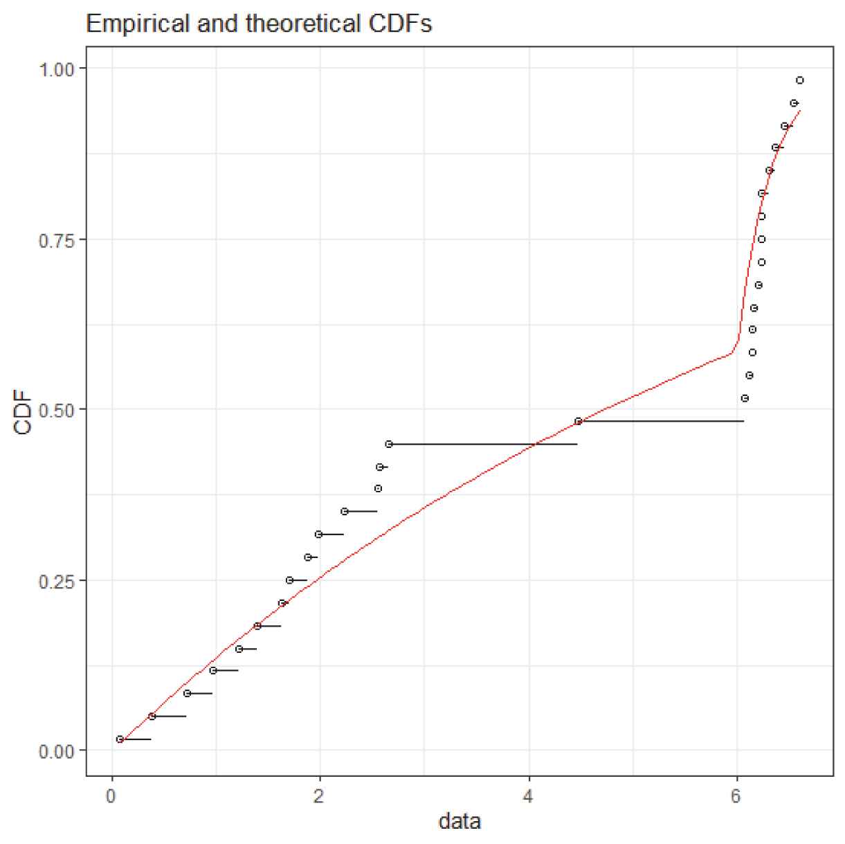
The empirical CDF (dots); and the estimated CDF based on MLE (solid line).
Suppose the life test ended when the 30-th lifetime is observed, i.e., we observe a Type-II censored sample with
First we compute the MLEs of
| s | True Value | MLP | CMP | 95% Pivotal PI | 95% HCD PI |
|---|---|---|---|---|---|
| 31 | 6.73 | 6.600 | 6.664 | (6.602, 6.973) | (6.600, 6.862) |
| 32 | 6.75 | 6.669 | 6.769 | (6.623, 7.236) | (6.607, 7.134) |
| 33 | 6.80 | 6.743 | 6.896 | (6.664, 7.539) | (6.644, 7.435) |
| 34 | 6.84 | 6.825 | 7.053 | (6.722, 7.918) | (6.706, 7.830) |
| 35 | 6.92 | 6.922 | 7.251 | (6.800, 8.424) | (6.793, 8.381) |
Point and interval prediction for future lifetimes of
7. CONCLUSION
In this paper, we have addressed the ALTs under CEM Type-II censoring Lomax data to produce the failure time data of highly reliable units in specified conditions. Under this setup, we have considered the estimation problem of the model parameters using the maximized likelihood and bootstrap methods. Further, point prediction by using the maximum likelihood prediction and conditional median prediction methods are also addressed. The PIs including pivot and conditional highest density arguments are considered. It is observed via MC simulation studies that the CIs based on the bootstrap method are more valid than the CIs based on the asymptotic normality method. In the prediction front, the CMP as a point predictor and highest conditional density prediction interval outperform the MLP and pivot prediction interval, respectively.
CONFLICTS OF INTEREST
The authors declare that there is no conflict of interest.
AUTHORS' CONTRIBUTIONS
The first author performed the writing up of the material, checking and conducting the numerical simulation while the second author developed the models, methodology and editing of the paper.
ACKNOWLEDGMENTS
The authors are grateful to the editor and referees for their comments and helpful suggestions.
REFERENCES
Cite this article
TY  - JOUR
AU  - Mohammad A. Amleh
AU  - Mohammad Z. Raqab
PY  - 2021
DA  - 2021/04/12
TI  - Inference in Simple Step-Stress Accelerated Life Tests for Type-II Censoring Lomax Data
JO  - Journal of Statistical Theory and Applications
SP  - 364
EP  - 379
VL  - 20
IS  - 2
SN  - 2214-1766
UR  - https://doi.org/10.2991/jsta.d.210406.001
DO  - 10.2991/jsta.d.210406.001
ID  - Amleh2021
ER  -