
The Kumaraswamy Marshall-Olkin Log-Logistic Distribution with Application
- DOI
- 10.2991/jsta.2018.17.1.5How to use a DOI?
- Keywords
- Kumaraswamy-G; Maximum likelihood; Log-Logistic; Order statistic
- Abstract
In this paper, we define and study a new lifetime model called the Kumaraswamy Marshall-Olkin log-logistic distribution. The new model has the advantage of being capable of modeling various shapes of aging and failure criteria. The new model contains some well-known distributions as special cases such as the Marshall-Olkin log-logistic, log-logistic, lomax, Pareto type II and Burr XII distributions. Some of its mathematical properties including explicit expressions for the quantile and generating functions, ordinary moments, skewness, kurtosis are derived. The maximum likelihood estimators of the unknown parameters are obtained. The importance and flexibility of the new model is proved empirically using a real data set.
- Copyright
- Copyright © 2018, the Authors. Published by Atlantis Press.
- Open Access
- This is an open access article under the CC BY-NC license (http://creativecommons.org/licences/by-nc/4.0/).
1. Introduction
There has been an increased interest in defining new generated classes of univariate continuous distributions by introducing additional shape parameter(s) to a baseline model. The extended distributions have attracted several statisticians to develop new models. The addition of parameters has been proven to be useful in exploring skewness and tail properties, and also for improving the goodness-of-fit of the generated family. The well-known generators are the following: the Marshall-Olkin distribution family by Marshall and Olkin (1997), the beta-G by Eugene et al. (2002), the Kumaraswamy-G (Kw-G) by Cordeiro and de Castro (2011), the Logistic-G by Torabi and Montazari (2014), the transformed-transformer (T-X) by Alzaatreh et al. (2013), the odd exponentiated generalized by Cordeiro et al. (2013), the Weibull-G by Bourguignon et al. (2014), the Kumaraswamy Marshal-Olkin distribution family by Alizadeh et al. (2015), the transmuted geometric-G by Afify et al. (2016a) and the beta transmuted-H by Afify et al. (2017).
Marshall and Olkin (1997) proposed a flexible family of distributions and introduced an interesting method of adding a new parameter to an existing distribution. The resulting new distribution includes the original distribution as a special case and gives more flexibility to model various types of data. For further information about the Marshall–Olkin family of distributions, see Barreto-Souza et al. (2013). The log-logistic (LL) distribution (known as the Fisk distribution in economics) has been widely used particularly in survival and reliability over the last few decades. It is the probability distribution of a random variable whose logarithm has a logistic distribution, an alternative to the log-normal distribution since it presents a failure rate function that increases initially and decreases later. The cumulative distribution function (cdf) and probability density function (pdf) of the LL distribution are given (for x > 0) by
Searching a more flexible LL distribution, many authors defined generalizations and modified forms of the LL distribution, with different number of parameters. For example, the Kumaraswamy log-logistic (de Santana et al., 2012), Marshall-Olkin LL (MOLL) (Gui, 2013), Lomax log-logistic (Cordeiro et al., 2014), McDonald log-logistic (Tahir et al., 2014), beta log-logistic (Lemonte, 2014), transmuted log-logistic (Granzotto and Louzada, 2015), Kumaraswamy transmuted log-logistic (Afify et al., 2016b) and generalized transmuted log-logistic (GTLL) (Nofal et al., 2017) distributions.
Gui (2013) defined the cdf and pdf of the MOLL distribution (for x > 0) by
The goal of this paper is to define and study a new lifetime model called the Kumaraswamy Marshall-Olkin Log-Logistic (“KMOLL” for short) distribution. The main feature of this model is that two additional shape parameters are inserted in (2) to give more flexibility in the form of the generated distribution. Based on the Kumaraswamy-generalized (K-G) family proposed by Cordeiro and de Castro (2011), we construct the new five-parameter KMOLL distribution. We give some mathematical properties of the new distribution with the hope that it will attract wider applications in engineering, reliability, life testing and other research. In fact, the KMOLL distribution can provide better fits than other models.
Let g(x) and G(x) denote the pdf and cdf of the baseline model. Cordeiro and de Castro (2011) defined the cdf of the K-G family by
To this end, we start from the MOLL distribution to define the new KMOLL distribution by inserting (1.2) in equations (1.3) and (1.4). Then, the cdf (for x > 0) of the KMOLL distribution is given by
A random variable X with the pdf (1.6) is denoted by X ~ KMOLL(a,b,α,γ,β). The survival function, hazard rate function (hrf) and cumulative hazard rate function (chrf) of X are, respectively, given by
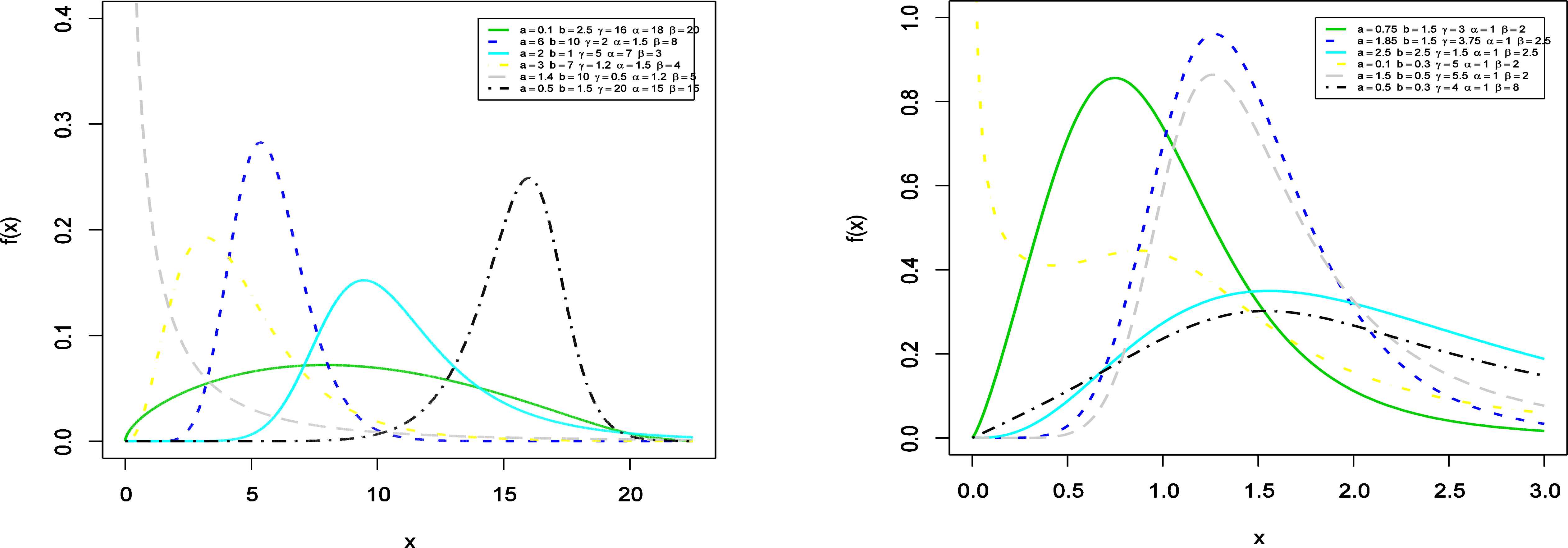
Plots for the pdf of the KMOLL distribution for several parameter values.
Plots for the hrf of the KMOLL distribution for several parameter values are displayed in Figure 2. Figure 2 shows that the hrf of the KMOLL distribution can be bathtub, upside down bathtub (unimodal), increasing or decreasing. This attractive flexibility makes the hrf of the KMOLL useful and suitable for non-monotone empirical hazard behaviors which are more likely to be encountered or observed in real life situations.
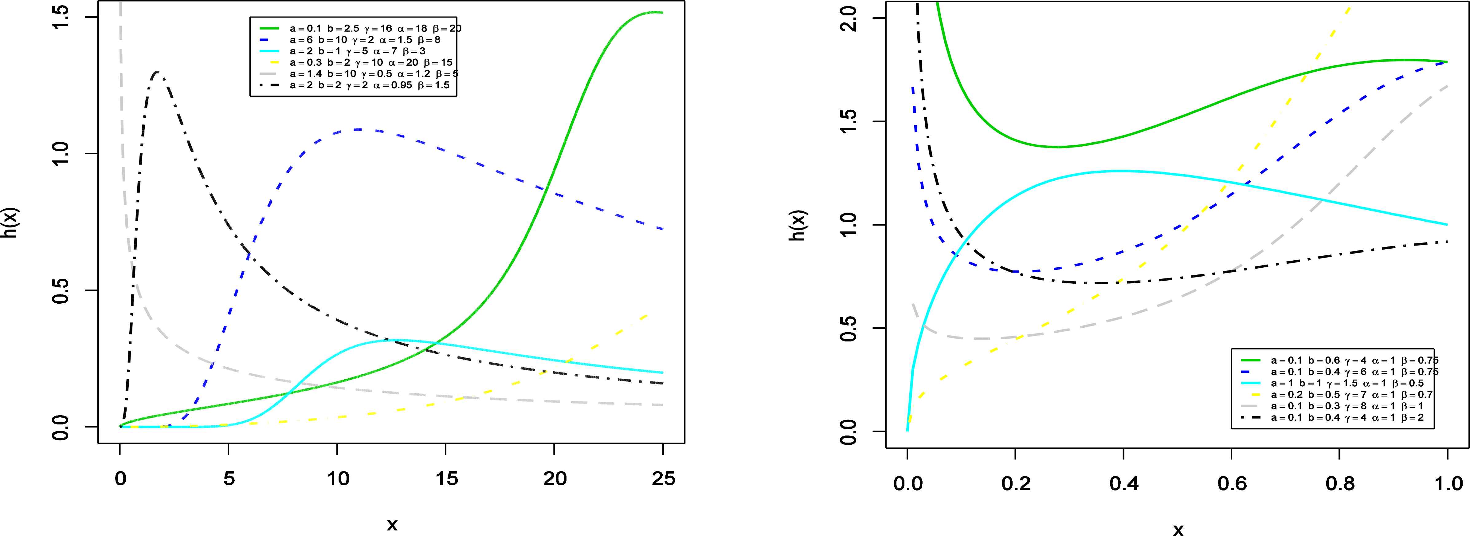
Plots of the hrf of the KMOLL distribution for several parameter values.
We now state a useful expansion for the KMOLL density. Using the binomial expansion, the pdf of the KMOLL reduces to
The importance of the KMOLL distribution is that it contains as special sub-models several well-known distributions. Table 1 lists the special distributions related to KMOLL distribution.
| Reduced Model | a | b | γ | α | β |
|---|---|---|---|---|---|
| KLL | a | b | γ | α | 1 |
| MOLL | 1 | 1 | γ | α | β |
| EMOLL | a | 1 | γ | α | β |
| GMOLL | 1 | b | γ | α | β |
| ELL | a | 1 | γ | α | 1 |
| GLL | 1 | b | γ | α | 1 |
| LL | 1 | 1 | γ | α | 1 |
| Dagum | a | 1 | γ | - | αβ1/γ |
| BurrXII | 1 | b | 1 | - | αβ |
| EBurrXII | a | b | 1 | - | αβ |
| ParetoII | 1 | 1/ b | 0 | - | αβ/b |
| EParetoII | a | 1/ b | 0 | - | αβ/b |
| Lomax | a | 1/ b | - | - | αβ/b |
Sub-models of the KMOLL distribution
The rest of the article is outlined as follows. In Section 2, we obtain the quantile function, shapes, skewness, kurtosis, moments, moment generating functions, Rényi entropies, reliability function and order statistics of X. Certain characterizations are presented in Section 3. The maximum likelihood estimates (MLEs) of the model parameters are obtained in Section 4. An application to real data set is considered in Section 5. Finally, Section 6 provides some concluding remarks.
2. The KMOLL Properties
In this section, we investigate mathematical properties of the KMOLL distribution including quantile function, skewness, kurtosis, shapes of functions, moments, the Rényi and Shannon entropies, reliability and order statistics.
2.1. Quantile function
Quantile functions are in widespread use in statistics and often find representations in terms of lookup tables for key percentiles. Let X ~ KMOLL(a,b,α,γ,β). The quantile function say Q(u) is defined by inverting F(x) in (1.5) as
2.2. Moments and moment generating function
Some of the most important features and characteristics of a distribution can be studied through moments (e.g. tendency, dispersion, skewness and kurtosis). Now we obtain ordinary moments and the moment generating function of the KMOLL distribution. The ordinary moments E(X)n = μ′n, n = 1,2,..., of the KMOLL distribution can be obtained, using (1.7), as
Further, the central moments (μn) and cumulants (κn), n = 1, 2,..., of the KMOLL distribution can be obtained from
The skewness
| KMOLL(a, b, γ, α, β) | μ′1 | μ′2 | μ′3 | μ′4 | S | K |
|---|---|---|---|---|---|---|
| (0.1,1.98,16,18,20) | 11.806 | 167.936 | 2656.865 | 45090.060 | 0.000 | −0.811 |
| (5,10,2,3,8) | 11.362 | 133.290 | 1612.749 | 20108.035 | 0.335 | 0.357 |
| (2,1,5,4,3) | 6.228 | 47.418 | 526.448 | 185560.800 | 4.883 | 2403.251 |
| (4,9,1.2,1.5,8) | 10.148 | 119.066 | 1601.209 | 24581.778 | 1.028 | 2.180 |
| (0.4,15,0.5,1.2,5) | 0.018 | 0.002 | 0.000 | 0.000 | 5.511 | 53.883 |
| (7,2,3.5,3,0.2) | 0.565 | 0.356 | 0.258 | 0.230 | 2.200 | 13.764 |
| (1,4,1,8,1) | 0.807 | 0.668 | 0.567 | 0.491 | −0.207 | 0.262 |
| (0.5,9,16,1,13) | 4.126 | 86.379 | 4204.147 | 381961.900 | 5.671 | 63.640 |
| (1.5,2.5,2,7,4) | 4.163 | 17.806 | 78.167 | 352.098 | 0.303 | 0.765 |
| (25,10,0.5,1.2,1) | 3.660 | 15.332 | 73.762 | 409.965 | 1.287 | 3.412 |
Moments, skewness and kurtosis of the KMOLL distribution for some parameter values
Table 2 indicates that the skewness value can be positive and negative, also close to zero. Hence, the KMOLL distribution can be right-skewed, left-skewed or symmetric.
Figure 3 also depicts plots for the skewness and kurtosis coefficients related to additional parameters. In the figure, a parameter decreases while other parameters are kept fixed. These plots indicate that both measures can be very sensitive on these shape parameters. Thus, indicating the importance of the proposed distribution.

Skewness and kurtosis plots of the KMOLL distribution for some parameter values
The moment generating function (mgf) is widely used as an alternative way to analytical results compared with working directly with pdf and cdf. The mgf of X is
Then we obtain
2.3. Unimodality
The pdf of the KMOLL model is decreasing or unimodal. In order to investigate the critical points of its density function, its first derivative with respect to x is
2.4. Entropies
The entropy of a random variable X with density function f(x) is a measure of variation of the uncertainty. Two popular entropy measures are the Rényi and Shannon entropies (Rényi (1961). Shannon (1951)). Here. we derive expressions for the Rényi and the Shannon entropies of the KMOLL distribution. The Rényi entropy of a random variable with pdf f(x) is defined as
The integral part of (2.5) is
Similarly, the following expectations are defined for (12) as
2.5. Reliability
In the context of reliability. the stress-strength model describes the life of a component which has a random strength X1 that is subjected to a random stress X2 The component fails at the instant that the stress applied to it exceeds the strength. and the component will function satisfactorily whenever X1 > X2. Hence, R = Pr(X2 < X1 ) is a measure of component reliability. Here. we obtain the reliability R when X1 ~ KMOLL(a1,b1,α,γ,β) and X2 ~ KMOLL(a2,b2,α,γ,β) are independent random variables. Probabilities of this form have many applications especially in engineering concepts.
Let fi and Fi denote the pdf and cdf Xi for i = 1,2,…,. Then, the reliability function for the KMOLL distribution is given by
2.6. Order statistics
Order statistics make their appearance in many areas of statistical theory and practice. They enter in the problems of estimation and hypotheses testing in a variety of ways. Therefore, we now discuss some properties of the order statistics for the proposed class of distributions. Let Xi:n denote the ith order statistic. Nadarajah et al. (2012) obtained the general results for the Kumaraswamy-G distribution. We use the results about the pdf fi:n(x) of the ith order statistic. Then. we can give the pdf fi:n(x) for a random sample X1, X2,…,Xn from the KMOLL distribution. It is well-known that
Several mathematical properties for the KMOLL order statistics (mgf, ordinary moments) can be derived from the mixture form in (2.9). Thus, from (2.9). the sth ordinary moment of Xi:n is given by
3. Characterizations
This section deals with various characterizations of KMOLL distribution. These characterizations are based on: (i) the ratio of two truncated moments; (ii) the hazard function and (iii) certain functions of the random variable. It should be mentioned that for characterization (i) the cdf need not have a closed form. We present our characterizations (i) − (iii) in three subsections.
3.1. Characterizations based on ratio of two truncated moments
In this subsection, we present characterizations of KMOLL distribution in terms of a simple relationship between two truncated moments. This characterization result employs a theorem due to (Glänzel. 1987). see Theorem 3.1 below. Note that the result holds also when the interval H is not closed. Moreover, as mentioned above. It could be also applied when the cdf F does not have a closed form. As shown in (Glänzel, 1990). This characterization is stable in the sense of weak convergence.
Theorem 3.1.
Let (Ω, F, P) Ω, be a given probability space and let H = [d,e] be an interval for some d < e (d = −∞, e = ∞ might as well be allowed). Let X: Ω → H be a continuous random variable with the distribution function F and let g and h be two real functions defined on H such that
Proposition 3.1.
Let X : Ω → (0, ∞) be a continuous random variable and let
Proof.
Let X be a random variable with pdf (1.6). Then,
Corollary 3.1.
Let X : Ω → (0, ∞) be a continuous random variable and let h(x) be as in Proposition 3.1. The pdf of X is (6) if and only if there exist functions g and ξ defined in Therorem 3.1 satisfying the differential equation
Remark 3.1.
For b = 1, (Mendoza et al., 2016). we let h(x) = g(x)[xβ + αβ]
−1
with g(x) = x−β(a−1). Then
The differential equation and general solution in this case are. respectively.
3.2. Characterization based on hazard function
It is known that the hazard function. hF. a twice differentiable distribution function, F, satisfies the first order differential equation
Proposition 3.2.
Let X : Ω → (0, ∞) be a continuous random variable. The pdf of X is (1.6) if and only if its hazard function hF (x) satisfies the differential equation
Proof.
If X has pdf (1.6) then clearly the above differential equation holds. Now, if it holds, then
Remark 3.2.
For a = b = 1 (special case of (1.4)). we have the following simple differential equation
3.3. Characterization based on certain functions of the random variable
The following propositions have already appeared in (Hamedani, 2013). so we will just state them here which can be used to characterize KMOLL distribution.
Proposition 3.3.
Let X : Ω → (d, e) be a continuous random variable with cdf F. Let ψ(x) be a differentiable function on (d, e) with limx→d+ ψ(x) = 1. Then for δ ≠ 1.
Remark 3.3.
It is easy to see that for certain functions. e.g.,
Proposition 3.3 provides a characterization of KMOLL distribution. Clearly there are other suitable functions ψ. We chose the above one for simplicity.
4. Maximum Likelihood Estimation
Several approaches for parameter estimation have been proposed in the literature but the maximum likelihood method is the most commonly employed. Here we consider estimation of the unknown parameters of the KMOLL distribution by the method of maximum likelihood. Let x1, x2,..., xn be observed values from the KMOLL distribution with parameters a,b,γ,α and β. The log-likelihood function for (a,b,γ,α,β) is given by
The derivatives of the log-likelihood function with respect to the parameters a,b,γ,α and β are given by respectively.
5. An Illustrative Application
In this section, we use a real data set to compare the fits of the KMOLL distribution with MOLL, LL and Weibull Fréchet (WFr) (Afify et al., 2016c) distributions. We will use a data set consists of 63 observations of the strengths of 1.5 cm glass fibres (Smith and Naylor, 1987), originally obtained by workers at the UK National Physical Laboratory. Unfortunately, the measurement units are not given in their paper. We estimate the unknown parameters of the distributions by the maximum likelihood. Then, we provide the values of the following statistics: Akaike Information Criterion (AIC), Consistent Akaike Information Criterion (CAIC) and Bayesian Information Criterion (BIC).
In general, the smaller the values of these statistics, the better the fit to the data. Table 3 lists the MLEs of the parameters and the values of AIC, CAIC and BIC statistics.
| Distribution | Estimated Parameters (Standard Error) | AIC | CAIC | BIC | ||||
|---|---|---|---|---|---|---|---|---|
| KMOLL(a, b, γ, α, β) | 1.8355 (0.096) | 0.0028 (0.002) | 47.4236 (13.307) | 0.0588 (0.030) | 0.2786 (0.095) | 28.0861 | 29.1387 | 38.8018 |
| MOLL(γ, α, β) | 2.3267 (1.289) | 0.0353 (0.154) | 7.9260 (0.873) | 51.5799 | 51.9867 | 58.0093 | ||
| LL(γ, α) | 1.5262 (0.041) | 7.9260 (0.873) | 49.5799 | 49.7799 | 53.8662 | |||
| WFr(α, β, a, b) | 0.3865 (0.799) | 0.2436 (0.285) | 1.4762 (4.782) | 16.8561 (20.485) | 39.0 | 47.6 | 42.4 | |
MLEs and the values of AIC, CAIC and BIC statistics
Based on Table 3, it is clear that KMOLL distribution provides the overall best fit and therefore could be chosen as the more adequate model than other models for explaining the data set. Table 4 gives Cramer-von Misses (W) and Anderson Darling statistics (A) for the three models which are the KMOLL, MOLL and LL distributions. More information is provided by a histogram of the data given in Figure 4. Fitted lines in Figure 4 represent the KMOLL, MOLL, LL and WFr distributions. Figure 5 shows empirical cdf and the fitted cdfs. Finally, we give Q-Q plots for all fitted models. The figures also reveals that the KMOLL fits the data very well.
| A | W | |
|---|---|---|
| KMOLL(a, b, γ, α, β) | 0.0181403 | 0.127219 |
| MOLL(γ, α, β) | 0.4969404 | 2.748973 |
| LL(γ, α) | 0.4969402 | 2.748972 |
Cramer-von Misses and Anderson Darling statistics
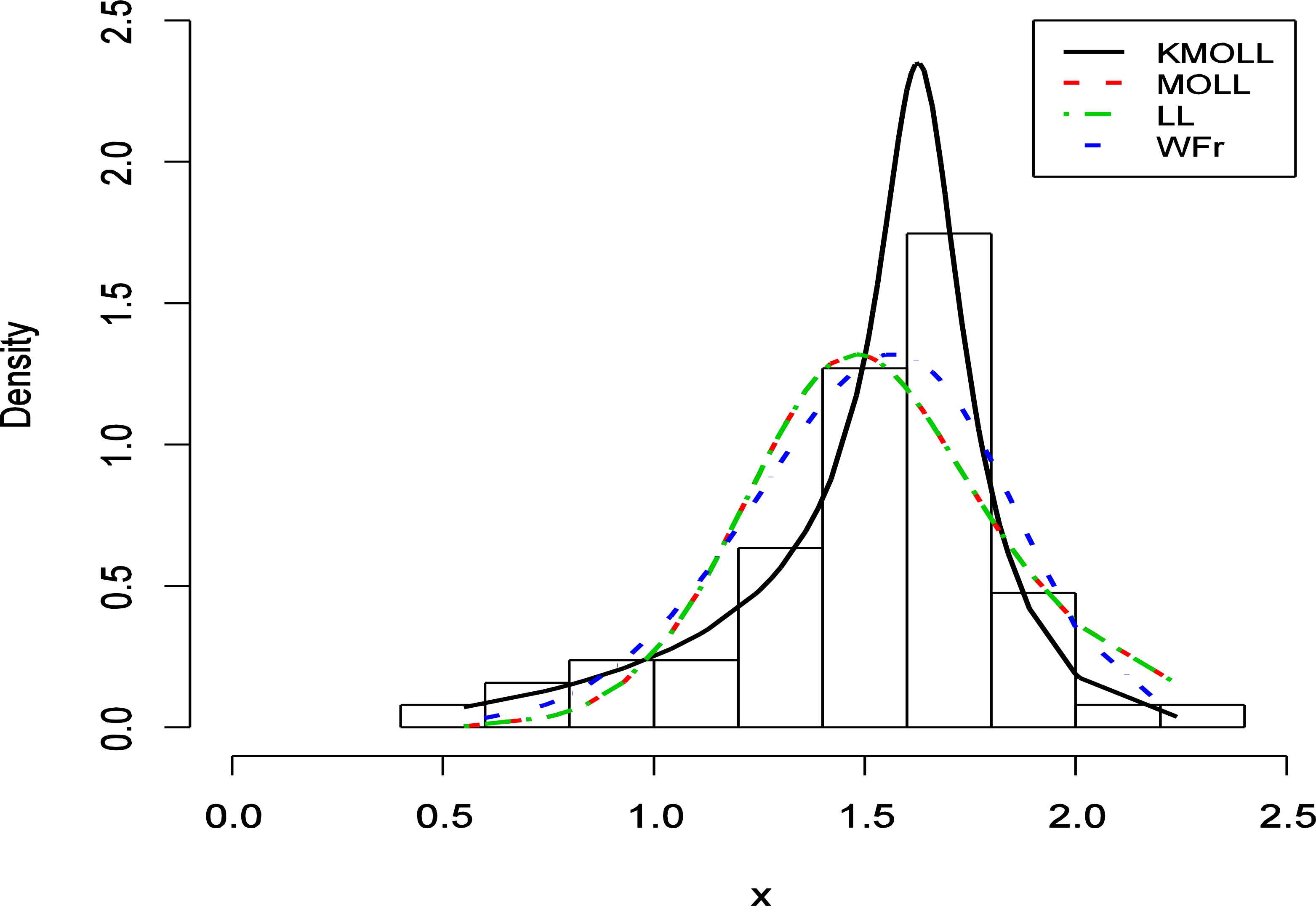
Fitted densities of the KMOLL, MOLL, LL and WFr distributions for the data set.
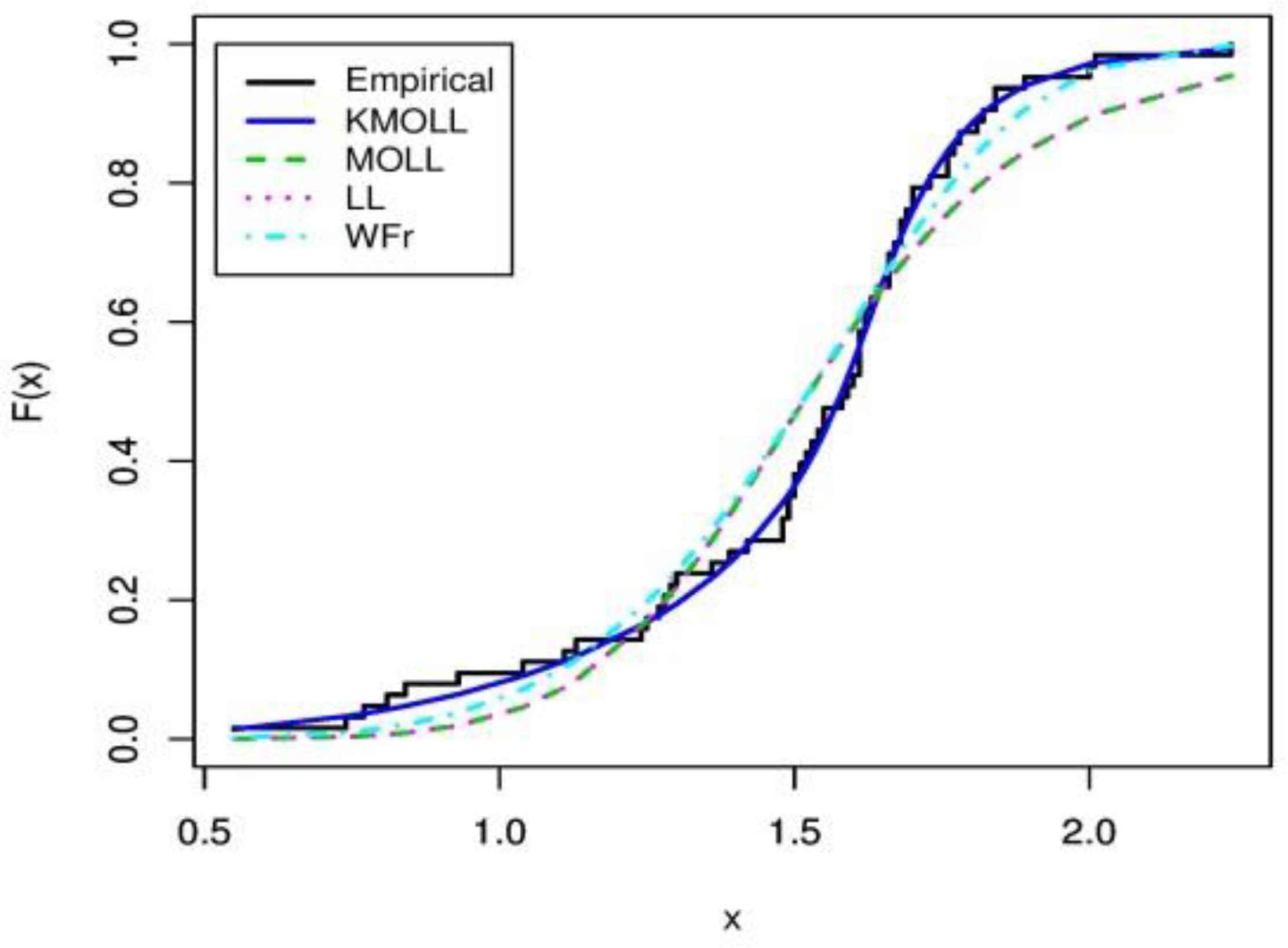
Estimated and KMOLL, MOLL, LL and WFr cdfs for the data set.
6. Conclusion
In this paper. we introduce a five-parameter distribution called the Kumaraswamy Marshal-Olkin log-logistic (KMOLL) distribution. Interestingly. our proposed model has increasing. upside-down bathtub and bathtub shaped hazard rate function. A study on the mathematical properties of the new distribution is presented. We obtain the moment generating function. ordinary moments. skewness. kurtosis. hazard and survival functions. The estimation of the model parameters is done via maximum likelihood method. We also provide a numerical example of our findings. We hope that the proposed model may attract applications in survival analysis and customer lifetime duration etc.
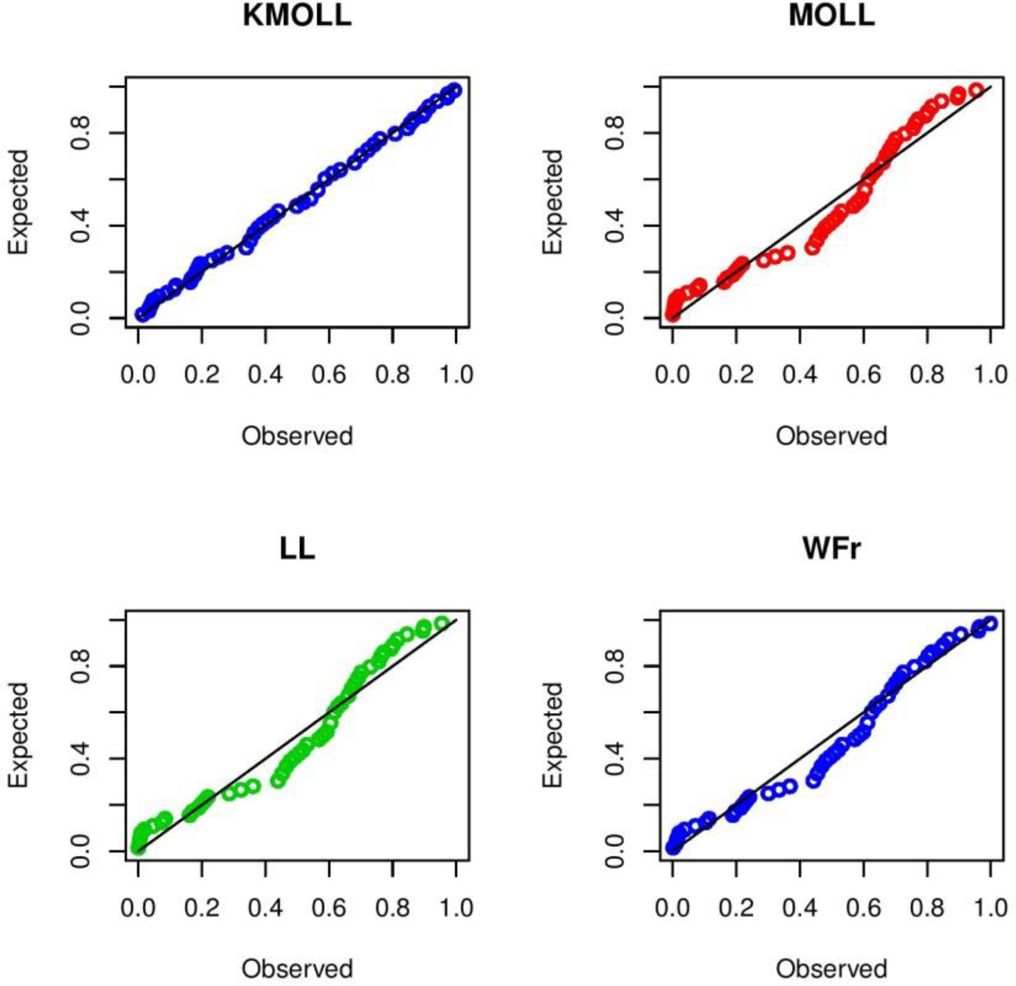
Q-Q plots for KMOLL, MOLL, LL and WFr distributions.
References
Cite this article
TY  - JOUR
AU  - Selen Cakmakyapan
AU  - Gamze Ozel
AU  - Yehia Mousa Hussein El Gebaly
AU  - G. G. Hamedani
PY  - 2018
DA  - 2018/03/31
TI  - The Kumaraswamy Marshall-Olkin Log-Logistic Distribution with Application
JO  - Journal of Statistical Theory and Applications
SP  - 59
EP  - 76
VL  - 17
IS  - 1
SN  - 2214-1766
UR  - https://doi.org/10.2991/jsta.2018.17.1.5
DO  - 10.2991/jsta.2018.17.1.5
ID  - Cakmakyapan2018
ER  -