
Odd Generalized Exponential Flexible Weibull Extension Distribution
- DOI
- 10.2991/jsta.2018.17.1.6How to use a DOI?
- Keywords
- Odd Generalized Exponential Family; Flexible Weibull Extension distribution; Generalized Weibull; Odd Generalized Exponential Flexible Weibull distribution; Maximum likelihood estimation
- Abstract
In this article we introduce a new four - parameters model called the odd generalized exponential flexible Weibull extension (OGE-FWE) distribution which exhibits bathtub-shaped hazard rate. Some of it’s statistical properties are obtained including ordinary and incomplete moments, quantile and mode, the moment generating functions, reliability and order statistics. The method of maximum likelihood is used for estimating the model parameters and the observed Fisher’s information matrix is given. Moreover, we give the advantage of the OGE-FWE distribution by an application using real data.
- Copyright
- Copyright © 2018, the Authors. Published by Atlantis Press.
- Open Access
- This is an open access article under the CC BY-NC license (http://creativecommons.org/licences/by-nc/4.0/).
1. Introduction
The Weibull distribution is a highly known distribution due to its utility in modelling lifetime data where the hazard rate function is monotone, [27]. Recently new classes of distributions were proposed based on modifications of the Weibull distribution to provide a good fit to data set with bathtub hazard failure rate, see [25]. Among of these, Exponentiated Weibull family, [14], Modified Weibull distribution, [11, 19], Beta-Weibull distribution, [8], A flexible Weibull extension, [4], Extended flexible Weibull, [4], Generalized modified Weibull distribution, [5], Kumaraswamy Weibull distribution, [6], Beta modified Weibull distribution, [16,22], Beta generalized Weibull distribution, [23], A new modified weibull distribution, [2] and Exponentiated modified Weibull extension distribution, [20], among others. A good review of these models is presented in [3,15,17].
The flexible Weibull extension (FWE) distribution, [4] has many applications in life testing experiments, reliability analysis, applied statistics and clinical studies. For more details on this distribution, see [4].
A random variable X is said to have the Flexible Weibull Extension (FWE) distribution with parameters α, β > 0 if it’s probability density function (pdf) is given by
If G(x), x > 0 is cumulative distribution function (cdf) of a random variable X, then the corresponding survival function is
This paper can be organized as follows, we define the cumulative, density and hazard functions of the odd generalized exponential flexible Weibull extension (OGE-FWE) distribution in Section 2. In Sections 3, we present some statistical properties including, quantile function and median, the mode, rth moment, skewness and kurtosis. In Sections 4, we introduce the moment generating function. The distribution of the order statistics is expressed in Section 5. The maximum likelihood estimation of the parameters is determined in Section 6. We use real data sets and analyzed it by an application in Section 7 and the results are compared with existing distributions. Finally, we present a conclusion in Section 8.
2. The Odd Generalized Exponential Flexible Weibull Extension Distribution
In this section we studied the four parameters odd generalized exponential flexible Weibull extension OGE-FWE (ϑ, γ, α, β) distribution. Using G(x) from Eq. (1.2) and g(x) from Eq. (1.1) to obtain the cdf and pdf of Eqs. (1.6) and (1.7), respectively. The cumulative distribution function cdf of the odd generalized exponential flexible Weibull extension distribution (OGE-FWE) is given by
The survival function S(x), hazard rate function h(x) and reversed hazard rate function r(x) of X ~ OGE-FWE (ϑ, γ, α, β) are given by
Figures (1–3) display the cdf, pdf, survival, hazard rate and reversed hazard rate function of the OGE-FWE (ϑ, γ, α,β) distribution for some parameter values.
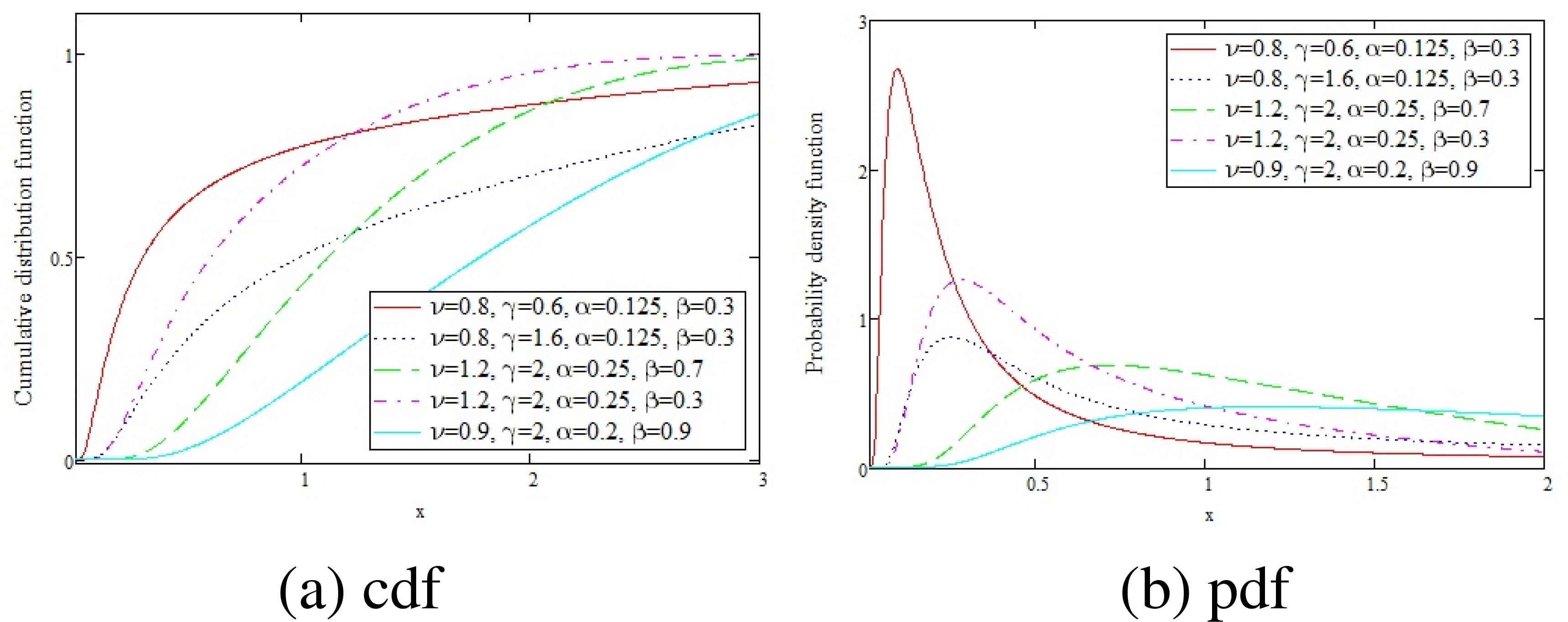
The cdf and pdf of the OGE-FWE for different values of parameters.
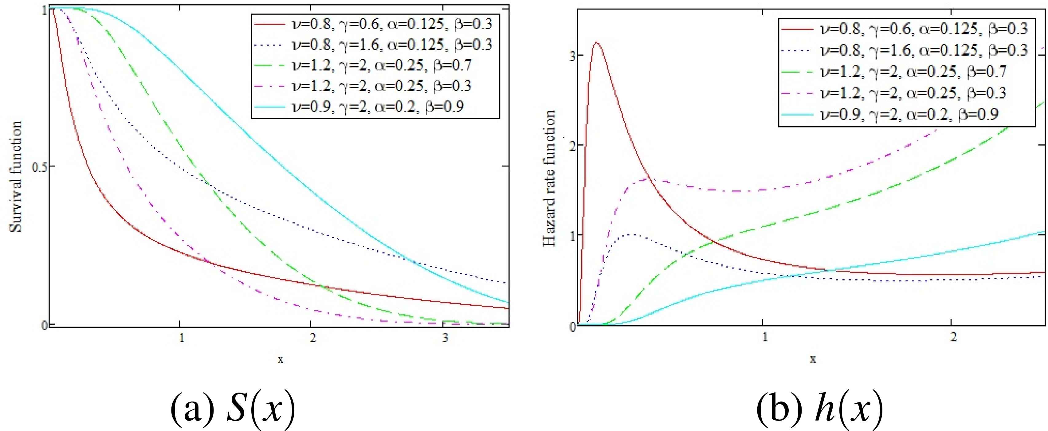
The survival and hazard rate functions of the OGE-FWE for different values of parameters.
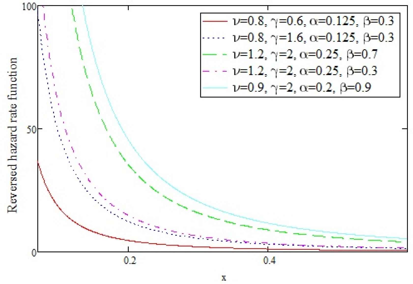
The reversed hazard rate function of the OGE-FWE for different values of parameters.
3. Statistical Properties
In this section, we will study some statistical properties for the OGE-FWE distribution, specially quantile function and simulation median, the mode, moments, skewness and kurtosis.
3.1. Quantile and median
We determine the explicit formulas of the quantile and simulation median of the OGE-FWE distribution. The quantile xq of the OGE-FWE(ϑ, γ, α, β) distribution is given by
3.2. The mode
In this subsection, we can obtain the mode of the OGE-FWE distribution by differentiating its probability density function pdf with respect to x and equaling it to zero. The mode is the solution the following equation
It is difficult to get an analytic solution in x to Eq. (3.6) in the general case. So, it has to be obtained by numerically methods.
3.3. Skewness and Kurtosis
In this subsection, we obtain the skewness and kurtosis based on quantile measures. The Moors Kurtosis is given by, [13]
3.4. The Moments
We derive the rth moment for the OGE-FWE distribution in Theorem (3.1)
Theorem 3.1.
If X has OGE-FWE (ϑ, γ, α, β) distribution, then The rth moments of random variable X, is given by
Proof.
We start with the well known distribution of the rth moment of the random variable X with probability density function f(x) given by
4. The Moment Generating Function
The moment generating function (mgf) of the OGE-FWE distribution is given by Theorem (4.1).
Theorem 4.1.
The moment generating function (mgf) of OGE-FWE distribution is given by
Proof.
The moment generating function MX(t) of the random variable X with probability density function f(x) is given by
5. Order Statistics
In this section, we derive closed form expressions for the PDFs of the rth order statistic of the OGE-FWE distribution. Let X1:n, X2:n,··· ,Xn:n denote the order statistics obtained from a random sample X1, X2, ··· , Xn which taken from a continuous population with cumulative distribution function cdf F(x; φ) and probability density function pdf f(x; φ), then the pdf of Xr:n is given as follows
Relation (5.3) show that fr:n(x; φ) is the weighted average of the OGE-FWE distribution with different shape parameters.
6. Parameters Estimation
In this section, point and interval estimation of the unknown parameters of the OGE-FWE distribution are derived by using the maximum likelihood method based on a complete sample.
6.1. Maximum Likelihood Estimation:
Let x1, x2,··· ,xn denote a random sample of complete data from the OGE-FWE distribution. The Likelihood function is given as
6.2. Asymptotic confidence bounds
In this section, we derive the asymptotic confidence intervals of these parameters when ϑ, γ, α > 0 and β > 0 as the MLEs of the unknown parameters ϑ, γ, α > 0 and β > 0 can not be obtained in closed forms, by using variance covariance matrix I −1 see [12], where I −1 is the inverse of the observed information matrix which defined as follows
7. Application
In this section, we will analysis of a real data set using the OGE-FWE (ϑ, γ, α, β) model and compare it with the other fitted models like a flexible Weibull extension distributions using Kolmogorov Smirnov (K-S) statistic, as well as Akaike information criterion(AIC), [?], Akaike Information Citerion with correction (AICC), Bayesian information criterion (BIC), Hannan-Quinn information criterion (HQIC) and Schwarz information criterion (SIC) values, [21]. The data have been obtained from [18], it is for the time between failures (thousands of hours) of secondary reactor pumps, Table 1.
| 2.160 | 0.746 | 0.402 | 0.954 | 0.491 | 6.560 | 4.992 | 0.347 |
| 0.150 | 0.358 | 0.101 | 1.359 | 3.465 | 1.060 | 0.614 | 1.921 |
| 4.082 | 0.199 | 0.605 | 0.273 | 0.070 | 0.062 | 5.320 |
Time between failures of secondary reactor pumps.
Table 2 gives MLEs of parameters of the OGE-FWE and K-S Statistics. The values of the log-likelihood functions, AIC, AICC, BIC, HQIC, and SIC are in Table 3.
| Model | K-S | |||||
|---|---|---|---|---|---|---|
| OGE-FWE | 0.2380 | 2.0700 | – | 0.069 | 0.113 | 0.0760 |
| Flexible Weibull | 0.0207 | 2.5875 | – | – | – | 0.1342 |
| Weibull | 0.8077 | 13.9148 | – | – | – | 0.1173 |
| Modified Weibull | 0.1213 | 0.7924 | 0.0009 | – | – | 0.1188 |
| Reduced Additive Weibull | 0.0070 | 1.7292 | 0.0452 | – | – | 0.1619 |
| Extended Weibull | 0.4189 | 1.0212 | 10.2778 | – | – | 0.1057 |
MLEs and K–S of parameters for secondary reactor pumps.
| Model | L | AIC | AICC | BIC | HQIC | SIC |
|---|---|---|---|---|---|---|
| OGE-FEW | −29.2980 | 66.5960 | 68.8182 | 71.1380 | 10.5590 | 71.1380 |
| Flexible Weibull | −83.3424 | 170.6848 | 171.2848 | 172.9558 | 12.5416 | 172.9558 |
| Weibull | −85.4734 | 174.9468 | 175.5468 | 177.2178 | 12.5915 | 177.2178 |
| Modified Weibull | −85.4677 | 176.9354 | 178.1986 | 180.3419 | 12.6029 | 180.3419 |
| Reduced additive Weibull | −86.0728 | 178.1456 | 179.4088 | 181.5521 | 12.6168 | 181.5521 |
| Extended Weibull | −86.6343 | 179.2686 | 180.5318 | 182.6751 | 12.6296 | 182.6751 |
Log-likelihood, AIC, AICC, BIC, HQIC and SIC values of models fitted.
Substituting the MLEs of the unknown parameters ϑ, γ, α, β into (6.7), we obtain estimation of the variance covariance matrix as the following
The nonparametric estimate of the survival function S(x) using the Kaplan-Meier method and its fitted parametric estimations when the distribution is assumed to be OGE-FWE, FW, W, MW, RAW and EW are computed and plotted in Figure 4.
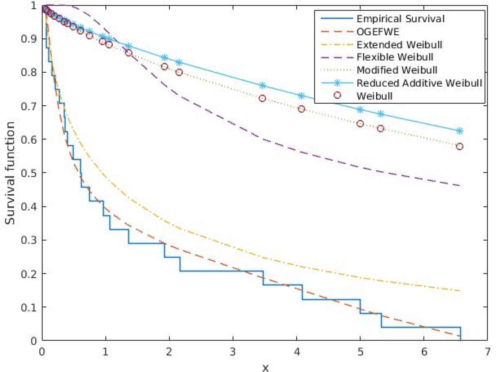
The Kaplan-Meier estimate of the survival function for the data.
Figure 5 gives the form of the hazard rate h(x) and cumulative density function cdf for the OGE-FWE, FW, W, MW, RAW and EW which are used to fit the data after the unknown parameters included in each distribution are replaced by their MLEs.
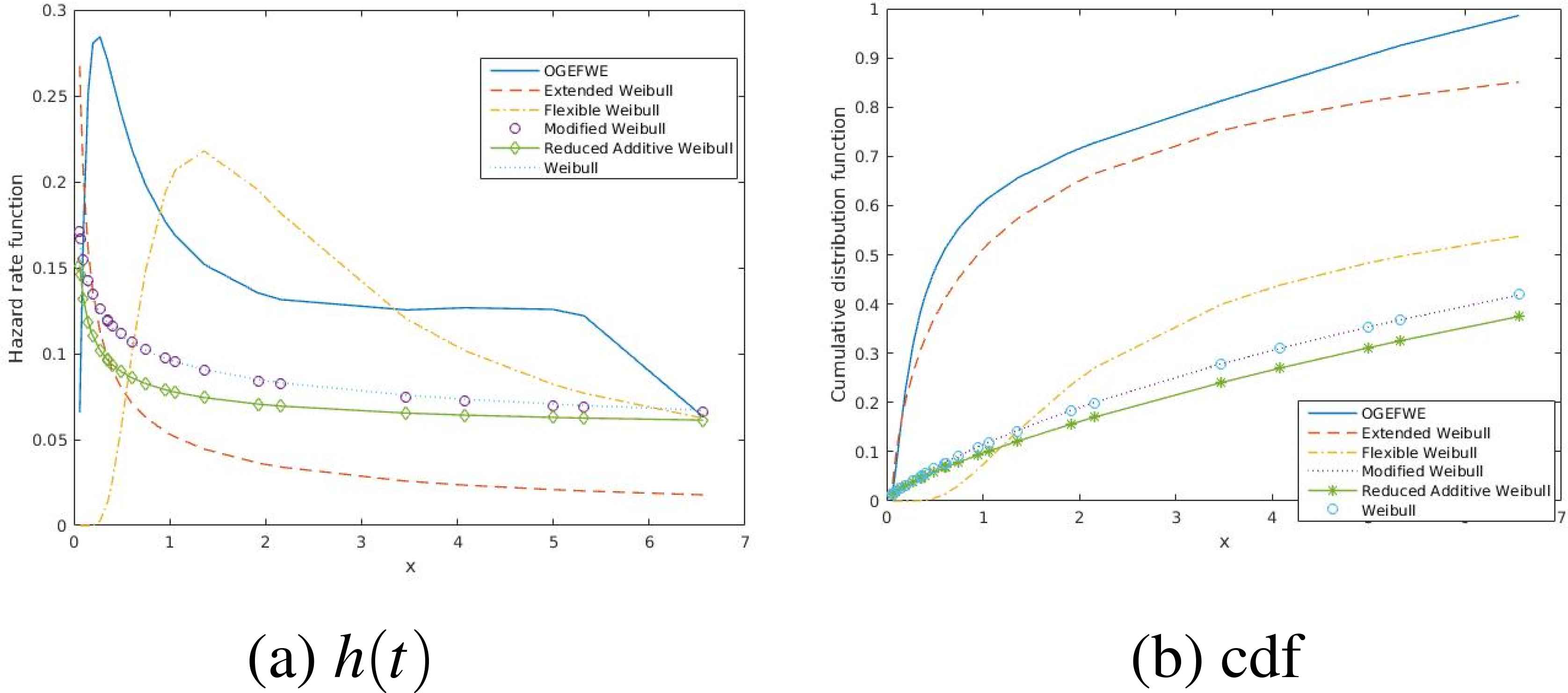
The Fitted hazard rate and cumulative distribution function for the data.
We find that the OGE-FWE distribution with the four - parameters provides a better fit than the previous new modified a flexible Weibull extension distribution(FWE) which was the best in [4]. It has the largest likelihood, and the smallest AIC, AICC, BIC, HQIC and SIC values among those considered in this paper.
8. Conclusions
We proposed a new distribution, based on odd generalized exponential family distributions, this distribution is named the odd generalized exponential flexible Weibull extension OGE-FWE distribution. Some its statistical properties are studied. The maximum likelihood method is used for estimating the parameters model. Finally, we introduce an application using real data. We show that the OGE-FWE distribution fits certain well known data sets better than existing modifications of the Weibull and flexible Weibull extension distributions.
References
Cite this article
TY  - JOUR
AU  - Abdelfattah Mustafa
AU  - Beih S. El-Desouky
AU  - Shamsan AL-Garash
PY  - 2018
DA  - 2018/03/31
TI  - Odd Generalized Exponential Flexible Weibull Extension Distribution
JO  - Journal of Statistical Theory and Applications
SP  - 77
EP  - 90
VL  - 17
IS  - 1
SN  - 2214-1766
UR  - https://doi.org/10.2991/jsta.2018.17.1.6
DO  - 10.2991/jsta.2018.17.1.6
ID  - Mustafa2018
ER  -