
On Some Aspects of a New Class of Two-Piece Asymmetric Normal Distribution
- DOI
- 10.2991/jsta.2018.17.1.8How to use a DOI?
- Keywords
- Method of maximum likelihood; Plurimodality; Probability density function; Skewness; Skew normal distribution
- Abstract
Through this chapter, we introduce a new class of two-piece asymmetric normal distribution suitable for asymmetric and plurimodal situations. We study some important aspects of this distribution by deriving explicit expressions for its distribution function, characteristic function, reliability measures etc. A location-scale extension of this class of distribution is considered and carried out the maximum likelihood estimation of its parameters. Further we have fitted the distribution to a real life data set for illustrating the usefulness of the model.
- Copyright
- Copyright © 2018, the Authors. Published by Atlantis Press.
- Open Access
- This is an open access article under the CC BY-NC license (http://creativecommons.org/licences/by-nc/4.0/).
1. Introduction
The term skew normal distribution (SND) refers to a parametric class of probability distribution that extends the normal distribution by an additional shape parameter which regulates skewness. The first systematic treatment of the SND in the scalar case was done by Azzalini (1985). He defined the SND as follows:
A random variable X is said to have skew normal distribution with skewness parameter θ ∈ R = (−∞, ∞), denoted by SND(θ), if its probability density function (p.d.f.) g1 (x; θ) is of the following form. For x ∈ R,
A random variable Y is said to follow the asymmetric normal distribution if its p.d.f. takes the following form. For y ∈ R,
For getting more flexible asymmetric normal models, some researchers recently studied two-piece versions of skew normal distributions. For example see Kim (2005), Jamalizadeh et. al (2012), Kumar and Anusree (2013) and Salehi et. al (2013). The main objective of the present article is to introduce a two-piece version of the AND(λ, α) as an asymmetric class of distribution suitable for tackling plurimodal situations. Throughout in this chapter we denote this class of distribution as “generalized two-piece asymmetric normal distribution (GTAND)”. The paper is organized as follows. In section 2 we present the definition of GTAND and derive some of its important properties. In section 3, we discuss some concepts regarding the mode of the distribution. In section 4, we obtain expression for certain reliability measures such as failure rate, reliability function and mean residual life function of the GTAND. A location-scale extension of the GTAND is considered in section 5 and obtained some of its important properties. Further, the parameters of the GTAND are estimated by method of maximum likelihood in section 6 and a numerical illustration is given in section 7.
We need the following shorter notation in the sequel. For any reals a, b and k such that bx + k > 0
2. Definition and Properties
In this section, first we define a wide class of two-piece asymmetric normal distribution and discuss some of its important properties.
Definition 1.
A random variable Z is said to follow a two-piece asymmetric normal distribution with parameters λ1, λ2 ∈ R = (−∞, ∞), α∈[0, 1] if its p.d.f. h(z; λ1, λ2, α) is of the following form. For z ∈ R,
Note that (4) is a proper probability density in the light of the following lemma.
Lemma 1.
If U is a standard normal variable, then for any real λ and k0,
Clearly, the GTAND(λ1, λ2, α) contains the following special cases.
- 1.
When λ1 = λ, λ2 = ρλ and α = 0, the distribution with p.d.f.(4) reduces to the two-piece skew normal distribution of Kumar and Anusree (2013)with parameters λ and ρ,
- 2.
when λ1 = λ, λ2 = λ, the distribution with p.d.f.(4) reduces to the skew normal distribution of Kumar and Anusree (2011b),
- 3.
when, λ1 → −∞, λ2 → ∞ or λ1 → −∞, λ2 → −∞, α = 1 or λ1 → ∞, λ2 → ∞, α = 1 or λ1 = 0, λ2 = 0 the distribution with p.d.f.(4) reduces to the standard normal distribution,
- 4.
- 5.
when either λ1 → −∞, λ2 → −∞, α = 2 or λ1 → ∞, λ2 → ∞, α = 0 TPSND(λ1, λ2, α), the distribution with p.d.f.(4) reduces to the half normal distribution.
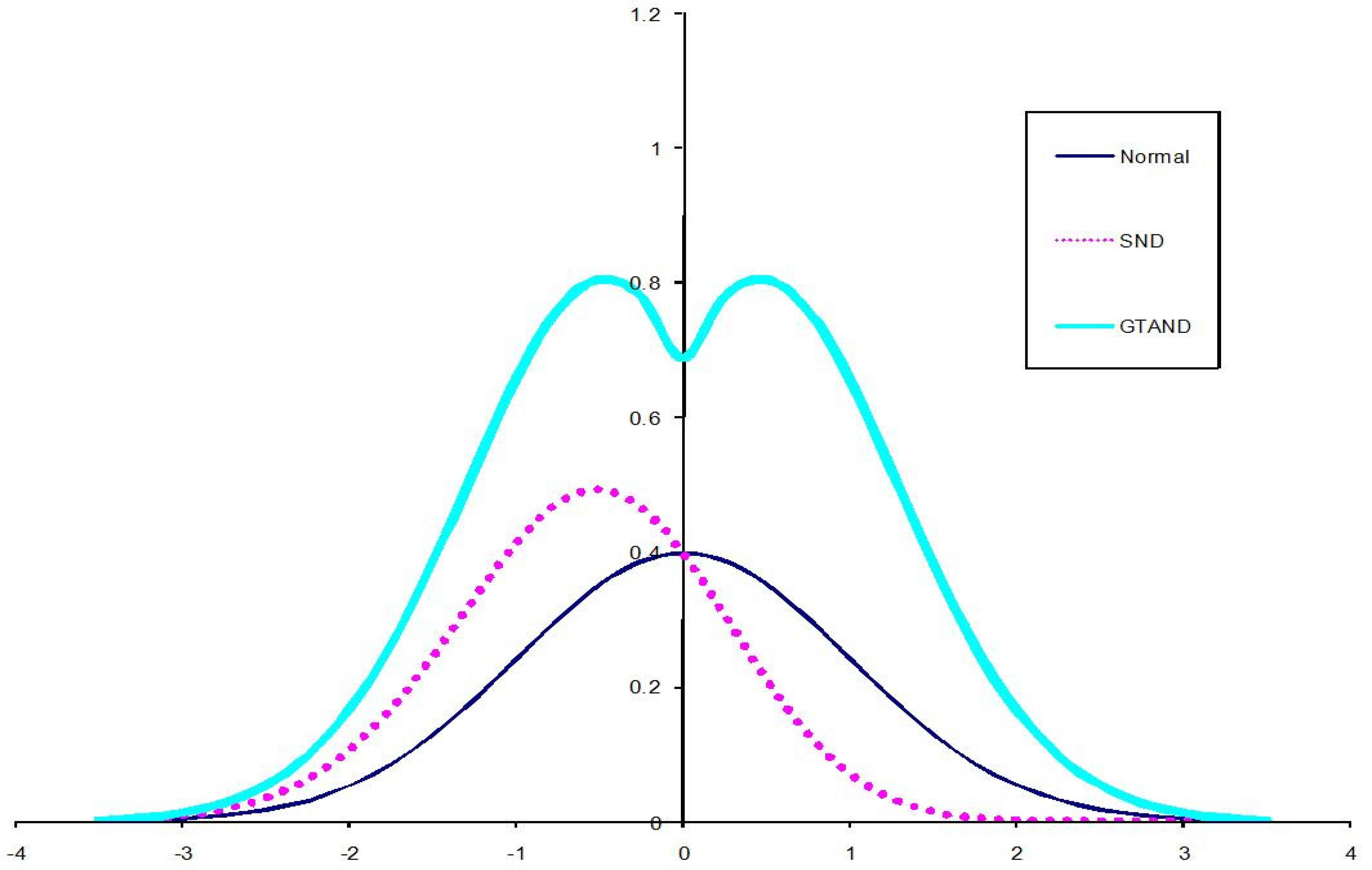
Probability plots of Normal, SND and GTAND

Probability plots of GTAND(−0.65, 0.65, α) for different choices of α = 0.1, 0.58, 0.78, 0.005.
Result 1.
If Z follows GTAND(λ1, λ2, α) with p.d.f. h(z; λ1, λ2, α), then Y1 = −Z follows GTAND(−λ2, − λ1, α).
Proof.
For any y1 ∈ R, the p.d.f. h1 (y1; λ1, λ2, α) of Y1 is given by
Result 2.
If Z follows GTAND(λ1, λ2, α) with p.d.f. h(z; λ1, λ2, α), then Z2 has p.d.f. (6).
Proof.
The p.d.f. h2 (y2; λ1, λ2, α) of Y2 is given by
Remark 1.
Note that when λ1 = 0 and λ2 = 0, (6) reduces to the p.d.f. of a Chi-square variate with one degree of freedom.
Result 3.
If Z is a GTAND(λ1, λ2, α) variate, then for any reals d1, d2 such that d1 ≤ d2,
Proof.
For any d1 ≤ d2 < 0, by definition,
Now, for the case 0 ≤ d1 ≤ d2,
Result 4.
The distribution function H (z; λ1, λ2, α) of a random variable Z with p.d.f. (4) is the following.
Proof.
Let Z be a random variable with p.d.f. (4) and H (z; λ1, λ2, α) be the cumulative distribution function. Then
In order to obtain the characteristic function of GTAND(λ1, λ2, α), we need the following lemma from Ellison (1964),
Lemma 2.
For any a1, a2 ∈ R and a standard normal variable Z with distribution function F
Result 5.
The characteristic function, ϕZ (t) of a random variable Z following GTAND(λ1, λ2, α) with p.d.f (4) is the following, for any t ∈ R and
Proof:
Let Z follows GTAND(λ1, λ2, α) with p.d.f. (4). By the definition of characteristic function, for any t ∈ R and
3. Mode
Result 6.
The p.d.f. of GTAND(λ1, λ2, α) is bimodal, if
- (1).
λ1 ≤ 0 and λ2 ≥ 0,
- (2).
λ1 ≤ 0 or λ2 < 0 provided and k3 (z; λ1, λ2, α) + k4 (z; λ1, λ2, α) ≤ 0,
- (3).
λ2 ≥ 0 or λ1 > 0 provided and k1 (z; λ1, λ2, α) + k2 (z; λ1, λ2, α) ≥ 0,
and
- (4).
λ1 > 0 and λ2 < 0 such that k1 (z; λ1, λ2, α) + k2 (z; λ1, λ2, α) ≥ 0 and k3 (z; λ1, λ2, α) + k4 (z; λ1, λ2, α) ≤0,
where
and
Proof:
In order to show that there exists unimodes in regions of z ∈ (−∞, 0] and z ∈ [0, ∞), it is enough to show that the second derivative of h(z; λ1, λ2, α) is negative for all α, λ1 and λ2 in the respective region.
For z ∈ (−∞, 0), we have
As a consequence of Result 6 we obtain the following result.
Result 7.
The p.d.f. of GTAND(λ1, λ2, α) is plurimodal, if
- (1)
λ1 ≤ 0 or λ2 < 0 provided and k3(z; λ1, λ2, α) + k4(z; λ1, λ2, α) > 0,
- (2)
λ2 ≥ 0 or λ1 > 0 provided and k1(z; λ1, λ2, α) + k2(z; λ1, λ2, α) < 0,
and
- (3)
λ1 > 0 and λ2 < 0 such that k1(z; λ1, λ2, α) + k2(z; λ1, λ2, α) > 0 and k3(z; λ1, λ2, α) + k4(z; λ1, λ2, α) < 0
4. Reliability aspects
Here we derive some properties of the GTAND(λ1, λ2, α), which are useful in reliability studies.
Let Z follows GTAND(λ1, λ2, α) with p.d.f.(4). Now from the definition of reliability function R(t; λ1, λ2, α) and failure rate r(t; λ1, λ2, α) of Z we obtain the following results.
Result 8.
The reliability function R(t; λ1, λ2, α) of Z following the GTAND(λ1, λ2, α) is
Proof follows from the definition of reliability function R(t; λ1, λ2, α) = 1− H(t; λ1, λ2, α) where H(t; λ1, λ2, α) is as given in Result.4.
Result 9.
The failure rate r(t; λ1, λ2, α) of Z following the GTAND(λ, α) is
Result 10.
The mean residual life function(MRLF) μ(t; λ1, λ2, α) of GTAND(λ1, λ2, α) is
Proof.
By definition, the MRLF of Z following the TAND(λ, α) is given by
5. Location-scale extension
In practical situation, the location-scale extension of GTAND(λ1, λ2, α) is more relevant. So in this section, we discuss the location-scale extension of the GTAND(λ1, λ2, α) and present some of its important properties similar to those we obtained for GTAND(λ1, λ2, α).
Definition 2.
Let Z follows GTAND(λ1, λ2, α), then X = μ + σZ is said to have an extended generalized two-piece asymmetric normal distribution with location parameter μ, scale parameter σ and shape parameters λ1, λ2 and α denoted as EGTAND(μ, σ; λ1, λ2, α), if its p.d.f. is given by
Clearly, the EGTAND(μ, σ; λ1, λ2, α) contains the following special cases.
- 1.
When λ1 = λ, λ2 = ρλ and α = 0, the distribution with p.d.f. (27) reduces to the location-scale extension of the two-piece skew normal distribution of Kumar and Anusree (2013),
- 2.
when λ1 = λ, λ2 = λ, the distribution with p.d.f. (27) reduces to the location-scale extension of the skew normal distribution of Kumar and Anusree (2011b),
- 3.
when, λ1 → −∞, λ2 → ∞ or λ1 → −∞, λ2 → −∞, α = 1 or λ1 → ∞, λ2 → ∞, α = 1 or λ1 = 0, λ2 = 0 the distribution with p.d.f. (27) reduces to normal distribution with parameters μ and σ,
- 4.
when λ1 = −λ, λ2 = λ and α = 0, the distribution with p.d.f. (27) reduces to location-scale extension of the skew normal distribution of Kim (2005) and
- 5.
when either λ1 → −∞, λ2 → −∞, α = 2 or λ1 → ∞, λ2 → ∞, α = 0 TPSND(λ1, λ2, α), the distribution with p.d.f. (27) reduces to the half normal distribution with parameters μ and σ.
Result 11.
The characteristic function ϕX (t) of a random variable X following EGTAND(μ, σ ; λ1, λ2, α) is the following, in which for each j = 1,2 and Sj = σitλj. For
Result 12.
The distribution function H (t) = H (t; μ, σ, λ1, λ2, α) of a random variable X following EGTAND(μ, σ; λ1, λ2, α) is the following,
Result 13.
The reliability function R(t) = R(t; μ, σ, λ1, λ2, α) of a random variable X following EGTAND(μ, σ ; λ1, λ2, α) is the following,
Result 5.4
The failure rate r(t) = r(t; μ, σ, λ1, λ2, α) of a random variable X following EGTAND(μ, σ; λ1, λ2, α) is the following,
6. Estimation
Let X1, X2 ,..., Xn be a random sample from EGTAND(μ, σ; λ1, λ2, α) with p.d.f. (27). Let X(1), X(2),...,X(n) be the ordered sample. Assume X(r) < μ < X(r+1), for a particular r=1,2,...,n. Then log-likelihood function of the sample is the following, in which ΣIj, denote the summation over the set Ij such that
7. Numerical computation
For a numerical illustration,we consider the following real life data set on the heights (in centimeters) of 100 Australian athletes, given in Cook and Weisberg (1994).The data recorded is as given below.
148.9 149 156 156.9 157.9 158.9 162 162 162.5 163 163.9 165 166.1 166.7 167.3 167.9 168 168.6 169.1 169.8 169.9 170
170 170.3 170.8 171.1 171.4 171.4 171.6 171.7 172 172.2 172.3 172.5 172.6 172.7 173 173.3 173.3 173.5 173.6 173.7 173.8
174 174 174 174.1 174.1 174.4 175 175 175 175.3 175.6 176 176 176 176 176.8 177 177.3 177.3 177.5 177.5 177.8 177.9
178 178.2 178.7 178.9 179.3 179.5 179.6 179.6 179.7 179.7 179.8 179.9 180.2 180.2 180.5 180.5 180.9 181 181.3 182.1
182.7 183 183.3 183.3 184.6 184.7 185 185.2 186.2 186.3 188.7 189.7 193.4 195.9.
This data has been recently used by Salehi et. al (2013) for establishing that “generalized skew two-piece skew normal distribution[ GSTPSt(λ1, λ2, ρ) ]”fits the data better than certain existing models. We obtained the MLE of the parameters of of N(μ, σ), the location-scale extension of SND(λ)[ ESND((μ, σ ;λ) ], the location-scale extension of TPSND(λ, ρ) [ETPSND(μ, σ ; λ, ρ)] of Kumar and Anusree (2013a), the location-scale extension of GSTPSt(λ1, λ2, ρ) of Salehi et. al (2013) [ EGSTPSt(μ, σ ; λ1, λ2, ρ) ] and EGTAND(μ, σ ; λ1, λ2, α) with the help of equations (6.7) to (6.11) and MATHCAD software. The values of loglikelihood( l ), the Akaike’s Information Criterion (AIC), the Bayesian Information Criterion (BIC) and the corrected Akaike’s Information Criterion (AICc) are also computed and presented in Table 1.
| Distribution: | Normal (μ, σ) | ESND (μ, σ, λ) | ETPSND (μ, σ; λ, ρ) | EGSTPSt (μ, σ; λ1, λ2, ρ) | EGTAND (μ, σ; λ1, λ2, α) |
|---|---|---|---|---|---|
| 174.594 | 174.58 | 173.657 | 167.056 | 173.01 | |
| 8.24 | 8.20 | 8.21 | 7.73 | 8.48 | |
| - | 0.0016 | −0.18 | 0.219,0.244 | −2.92,0.765 | |
| - | - | - | - | 2.28 | |
| - | - | 0.974 | −0.991 | - | |
| l | −352.318 | −352.318 | −349 | −348 | −347.64 |
| AIC | 708.64 | 710.64 | 706 | 706 | 703 |
| BIC | 713.85 | 718.45 | 716 | 705 | 704 |
| AICc | 708.76 | 710.89 | 706.49 | 706.68 | 704 |
Estimated values of the parameters and the corresponding l, AIC, BIC and AICc values for the fitted models-the N(μ, σ), the ESND((μ, σ ;λ), the ETPSND(μ, σ ; λ, ρ), the EGSTPSt(μ, σ ; λ1, λ2, ρ) and the EGTAND(μ, σ ; λ1, λ2, α).
From Table 1 we can see that EGTAND(μ, σ; λ1, λ2, α) gives a better fit to the data given to the existing models-N(μ, σ), ESND((μ, σ; λ), ETPSND(μ, σ; λ, ρ) and EGSTPSt(μ, σ; λ1, λ2, ρ).
References
Cite this article
TY  - JOUR
AU  - C. Satheesh Kumar
AU  - M.R. Anusree
PY  - 2018
DA  - 2018/03/31
TI  - On Some Aspects of a New Class of Two-Piece Asymmetric Normal Distribution
JO  - Journal of Statistical Theory and Applications
SP  - 101
EP  - 121
VL  - 17
IS  - 1
SN  - 2214-1766
UR  - https://doi.org/10.2991/jsta.2018.17.1.8
DO  - 10.2991/jsta.2018.17.1.8
ID  - SatheeshKumar2018
ER  -