
The Exponential Lindley Odd Log-Logistic-G Family: Properties, Characterizations and Applications
- DOI
- 10.2991/jsta.2018.17.3.10How to use a DOI?
- Keywords
- Exponential Lindley family; odd log-logistic family; mixture distribution family; maximum likelihood; moments; characterizations; generalized distribution family; mixture family
- Abstract
A new family of distributions called the exponential Lindley odd log-logistic G family is introduced and studied. The new generator generalizes three newly defined G families and also defines two new G families. We provide some mathematical properties of the new family. Characterizations based on truncated moments as well as in terms of the hazard function are presented. The maximum likelihood is used for estimating the model parameters. We assess the performance of the maximum likelihood estimators in terms of biases and mean squared errors by means of a simulation study. Finally, the usefulness of the family is illustrated by means of three real data sets. The new model provides consistently better fits than other competitive models for these data sets.
- Copyright
- © 2018, the Authors. Published by Atlantis Press.
- Open Access
- This is an open access article under the CC BY-NC license (http://creativecommons.org/licences/by-nc/4.0/).
1. Introduction
Recently, several families of continuous uni-variate distributions have been constructed by extending common families of continuous models. These generalized distributions give more flexibility by adding one or more parameters to the baseline model. Many classes can be cited such as the Marshall-Olkin-G family by Marshall and Olkin [25], transmuted exponentiated generalized-G family by Yousof et al. [34], Burr X-G by Yousof et al. [35], type I half-logistic family by Cordeiro et al. [12], Zografos-Balakrishnan odd log-logistic family of distributions by Cordeiro et al. [13], a new generalized two-sided family of distributions by Korkmaz and Genç [22], generalized odd log-logistic family by Cordeiro et al. [10], odd-Burr generalized family by Alizadeh et al. [4], beta Weibull G by Yousof et al. [36], exponentiated generalized-G Poisson family by Aryal and Yousof [8], type I general exponential class by Hamedani et al. [20] and beta transmuted-H by Afify et al. [2] among others.
Recently, Gleaton and Lynch [17] introduced a class of distributions called the odd log-logistic family with one extra shape parameter α > 0 with cumulative distribution function (cdf)
The goal of this paper is to introduce a new flexible and wider family of the distributions based on T–X family using the EL as the generator. The paper is organized as follows. The new family is introduced in Section 2. Some members and sub-families of the new family are introduced in Section 3. In Section 4, the series expansions for cdf and pdf of the new family are presented. In Section 5, some of its mathematical properties are derived. Section 6 deals with some characterizations of the new family. In Section 7, the maximum likelihood method is presented. In Section 8, a simulation study is performed to evaluate the efficiency of the Maximum Likelihood method. In Section 9, we illustrate the importance of the new family by means of three applications to real data sets. The paper is concluded in Section 10.
2. The new family
We define the new family by taking W [G(x; ξ)] = −log[1 − H(x; ξ)] and r(t) = gEL (t; β, θ). From (1.1), (1.2), (1.3) and (1.4), we introduce cdf and pdf of the new family as
3. Some special cases of the ELOLL-G family
The ELOLL-G family includes important sub-families. We mention these sub-families in Table (1). Also, the (2.1) and (2.2) will be most tractable when g(x) and G(x) have simple analytic forms. Here, we provide three special models of the ELOLL-G family. These special models generalize some well-known distributions reported in the literature. We note that since the cdf, pdf and hrf of any ELOLL-G distribution will be easily determined by (2.1), (2.2) and (2.4), we dont give them in following sub-sections.
| α | β | θ | Sub-family | References |
|---|---|---|---|---|
| 1 | − | − | Exponential Lindley-G | New |
| 1 | 1 | − | Lindley-G | Çakmakyapan and Ozel [9] |
| 1 | 0 | − | Lehmann Type II-G or Proportional hazard rate model | Gupta et al. [19] |
| − | 0 | − | Odd Burr-G or Lehmann Type II odd log-logistic-G | Alizadeh et al. [4] |
| − | 1 | − | Lindley odd log-logistic-G | New |
| 1 | 0 | 1 | G(x) | - |
Sub families of the ELOLL-G family.
3.1. The ELOLL-normal distribution
We define the ELOLL-normal (ELOLL-N) distribution from (2.2)
by taking
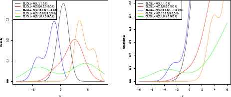
Plots of the pdf and hrf of the ELOLL-N distributions
3.2. The ELOLL-Weibull distribution
We now consider the Weibull distribution as a baseline distribution with pdf g(x; λ, γ) = γλγxγ−1e−(λx)γ and cdf G(x; λ, γ) = 1−e−(λx)γ for x, λ, γ > 0. Its pdf is denoted by ELOLL−W(Θ) where Θ = (α, β, θ, λ, γ). Its pdf and hrf for selected parameter values are displayed in Figure 2. From Figure 2, we see that pdf and hrf of the ELOLL-W model have various shapes. The pdf shapes are decreasing, unimodal, bi-modal, firstly decreasing then unimodal shaped, U-shaped. Also, its hrf shapes are increasing, decreasing, unimodal, bathtube-shaped and firstly unimodal and then increasing shaped. So, we can say that ELOLL-W distribution can be useful for modelling data.
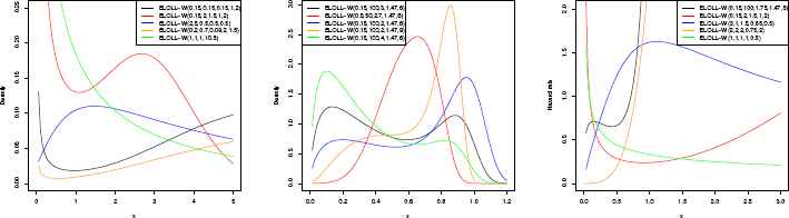
Plots of the pdf and hrf of the ELOLL-W distributions
3.3. The ELOLL-Lomax distribution
The pdf and cdf of the Lomax distribution with scale parameter λ > 0 and shape parameter k > 0 are given by
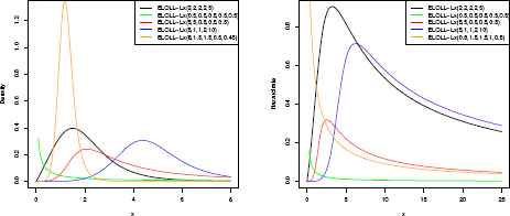
Plots of the pdf and hrf of the ELOLL-Lx distributions
4. Expansions for cdf and pdf
In this Section, we will obtain cdf and pdf expansions of the ELOLL-G family using Taylor series of
5. Properties
The rth moment of X, say µ′r, follows from (4.2) as
Using the series expansion
Suppose X1,...,Xn is a random sample from an ELOLL-G distribution. Let Xi:n denote the ith order statistic. The pdf of Xi:n can be expressed as
6. Characterizations
This section deals with various characterizations of ELOLL distribution. These characterizations are presented in two directions: (i) based on truncated moments and (ii) in terms of the hazard function. It should be noted that characterization (i) can be employed also when the cdf does not have a closed form. We present our characterizations (i) and (ii) in two subsections.
6.1. Characterizations based on truncated moments
Our first characterization employs a theorem due to Glanzel [16], see Theorem 1 of Appendix B. The result, however, holds also when the interval H is not closed since the condition of Theorem 1 is on the interior of H.
Proposition 1.6
Let X : Ω → ℝ be a continuous random variable and let
Corollary 1.6.
Let X : Ω → ℝ be a continuous random variable and let q1 (x) be as in Proposition 1. 6. The pdf of X is (2.2) pdf if and only if there exist functions q2 and η defined in Theorem 1 satisfying the differential equation
6.2. Characterization in terms of the hazard function
It is known that the hazard function, hF, of a twice differentiable distribution function, F, satisfies the first order differential equation
Proposition 2.6
Let X : Ω → ℝ be a continuous random variable. Then, for β = 0, X has pdf (2.2) if and only if its hazard function hF (x) satisfies the differential equation
7. Maximum Likelihood Estimation (MLE) and Inference
Several approaches for parameter estimation were proposed in the literature but the maximum likelihood method is the most commonly employed. The MLEs enjoy desirable properties and can be used for constructing confidence intervals and also for test statistics. The normal approximation for these estimators in large samples can be easily handled either analytically or numerically. Here, we consider the estimation of the unknown parameters of the new family from complete samples only by maximum likelihood. Let x1,...,xn be a random sample from ELOLL-G model with a (q+3)×1 parameter vector Ξ =(α, β, θ, ξ) ⊤ , where ξ is a q×1 baseline parameter vector. The log-likelihood function for Ξ can be expressed as
The likelihood ratio (LR) statistic can be used for comparing the some sub-models of ELOLLG model. For example, the LR statistic can be used to discriminate between the ELLOL-Lomax and L-Lomax since they are nested models, which is equivalently to test H0 : α = β = 1. The LR statistic reduces to
8. A simulation study
In this subsection, we perform the simulation study using the exponential Lindley odd log-logistic exponential distribution (ELOLL-E) which is the generalization of the exponential distribution with cdf F (x; λ) = 1 − exp(−λx), x > 0, λ > 0. To see the performance of MLE’s of this distributions, we generate 1,000 samples of sizes 20, 50 and 100 from ELOLL-E using inverse of the its cdf for θ = 2. The results of the simulation are reported in Table (2). From this Table, we observe that the estimates approach true values as the sample size increases whereas the standard devations of the estimates decrease.
| Parameters | n = 20 | n = 50 | n = 100 |
|---|---|---|---|
| α, β, λ | |||
| 1,1,1 | 1.0899,1.1654,1.0906 | 1.0170,1.0452,1.0189 | 1.0111,1.0031,0.9847 |
| (0.2581),(0.9818),(0.3488) | (0.1379),(0.8293),(0.2274) | (0.0848),(0.7345),(0.1670) | |
| 2,2,2 | 2.1705,2.3459,1.9854 | 2.0673,1.9774,1.9883 | 2.0361,1.9851,1.9916 |
| (0.4130),(1.9485),(0.2642) | (0.2550),(0.7811),(0.1546) | (0.1795),(0.5796),(0.1736) | |
| 2.1.0.5 | 2.1053,1.0154,0.5046 | 2.0586,1.0128,0.4996 | 2.0117,1.0085,0.5009 |
| (0.3937),(0.3690),(0.0603) | (0.2405),(0.3371),(0.0424) | (0.1653),(0.2717),(0.0286) | |
| 1,0.5,2 | 1.0147,0.7305,2.1798 | 1.0062,0.6800,2.0887 | 0.9945,0.6546,2.0635 |
| (0.2305),(0.8415),(0.7783) | (0.1214),(0.6699),(0.4054) | (0.0912),(0.5922),(0.4099) | |
| 1,2,0.5 | 1.0834,1.8239,0.5047 | 1.0284,1.9398,0.5030 | 1.0210,1.9620,0.5017 |
| (0.2335),(0.6285),(0.1195) | (0.1259),(0.4712),(0.0764) | (0.0872),(0.4550),(0.0530) | |
| 2,0.5,0,5 | 2.0795,0.5410,0.5105 | 2.0380,0.5515,0.5035 | 2.0156,0.5280,0.5033 |
| (0.3949),(0.2886),(0.0661) | (0.2302),(0.6220),(0.0445) | (0.1683),(0.5280),(0.0295) | |
| 0.75,5,2 | 0.8201,4.8903,2.1585 | 0.7895,4.8956,1.9550 | 0.7619,4.9821,1.9942 |
| (0.1484),(0.7185),(0.5310) | (0.1029),(0.3244),(0.3808) | (0.0659),(0.2595),(0.2433) | |
| 10,10,10 | 10.679,10.0500,10.0436 | 10.1903,10.0244,10.0041 | 10.1852,9.9983,9.9934 |
| (2.0187),(2.1032),(0.2139) | (1.1108),(1.5571),(0.1350) | (0.9405),(2.2128),(0.1038) | |
Emprical means and standard deviations (in paranthesis) for selected parameters values of ELOLL-E distribution
9. Data analysis
In this section, we introduce three applications using well-known data sets to show the flexibility and applicability of the proposed models over other models. First, we describe the data sets and we fit some distributions to these data sets using MLE method. Then we compare proposed distributions with several member of distribution families. The model selection is applied using the estimated log-likelihood (
First data set studied by Murthy et al. [27], which represent failure times for a particular windshield device. This data set has been analyzed by Cordeiro et al. [14]. Using this data set, we fit the ELOLL-N, Lindley-normal (L-N) (Çakmakyapan and Ozel, [9]), exponential-normal (E-N) or Lehmann type II exponentiated-normal (Alzaatreh et al., [5]; Cordeiro et al. [15]), McDonaldnormal (McN) (Alexander et al. [3]), normal-normal{exponential} (NNE) (Alzaatreh et al. [6]), normal-Cauchy{log-logistic} (NCLL) (Alzaatreh, et al. [7]), logistic-normal (LN) (Tahir et al. [32]), generelized Kumaraswamy-normal (GKw-N) (Cordeiro et al. [11]) and generalized odd log-logistic normal (GOLLN) (Cordeiro, et al. [10]) distributions models. The results of this application are listed in Table 3.
| Model | AIC,CAIC,BIC,HQIC | K-S (p-v.) | ||
|---|---|---|---|---|
| ELOLL-N | 0.1679, 6.5946, 3.0515, 3.1785, 0.4070 | 124.3870 | 258.7740, 259.5433, 270.9281, 263.6599 | 0.0463 |
| (0.0849), (9.5475), (0.6488), (0.2077), (0.1255) | (0.9937) | |||
| McN | 125.6276, 6.9936, 0.0299, 4.7966, 2.4578 | 128.2184 | 266.4367, 267.2059, 278.5908, 271.3225 | 0.0805 |
| (0.2334), (0.3941), (0.0131), (0.9119), (0.4754) | (0.6478) | |||
| NNE | 9.0338, 0.7306,−19.3314, 5.9635 | 128.4202 | 264.8404, 265.3467, 274.5637, 268.7491 | 0.0991 |
| (0.4896), (0.0873), –, (0.4711), (0.3606) | (0.3816) | |||
| NCLL | 14.6194, 0.7789,−19.0441, 4.4038 | 128.1291 | 264.2582, 264.7645 ,273.9814, 268.1669 | 0.0921 |
| (3.8058), (0.1874), –, (2.6534), (0.9849) | (0.4742) | |||
| LN | –, –, 6.1695, 1.1181, 4.0953 | 130.0301 | 266.0602, 266.3602, 273.3526, 268.9917 | 0.0805 |
| –, –,(4.5532), (1.0089), (3.0241) | (0.6482) | |||
| GKwN | 90.5274, 4.6255, 0.6399,−6.3998, 4.0251 | 127.9231 | 265.8463, 266.6155, 278.0003, 270.7321 | 0.0971 |
| (13.5280), (5.0395), (0.3384), (1.7059), (1.2968) | (0.4067) | |||
| GOLLN | 0.4557, 1.1863, –, 2.5139, 0.6358 | 127.0450 | 262.0900, 262.5963, 271.8133, 265.9987 | 0.0901 |
| (0.2353), (1.2905), –, (0.7508), (0.3306) | (0.5036) | |||
| L-N | –, –, 0.1446, 0.258, 0.5530 | 127.8708 | 261.7416, 262.0416, 269.0341, 264.6731 | 0.0775 |
| –, –, (0.0112), (1.3e-5), (6.2e-6) | (0.6946) | |||
| E-N | –, –, 0.1382, 1.0954, 0.5583 | 128.0645 | 262.1289, 262.4289, 269.4214, 265.0604 | 0.0618 |
| –, –, (0.0151), (0.0006), (0.0002) | (0.8908) |
MLEs of the model parameters for the windshield data, the corresponding standard errors (given in parentheses below estimated parameters) and the AIC, CAIC, BIC, HQIC and K-S values
As second data analysis, we analyze the data set studied by Abouammoh et al. [1], which represent the lifetime in days of 40 patients suffering from leukemia from one of the Ministry of Health Hospitals in Saudi Arabia. By using this data set we compare the ELOLL-W distribution with logistic-Weibull (LW) (Tahir et al. [32]), odd-Burr-Weibull (OBW) (Alizadeh et al. [4]), Lindley-Weibull (L-W) (Çakmakyapan and Ozel [9]) and exponential-Weibull (E-W) or ordinary Weibull distributions. The results of this application are listed in Table 4.
| Model | AIC,CAIC,BIC,HQIC | K-S(p-v.) | ||
|---|---|---|---|---|
| ELOLL-W | 0.2389, 44 1.841 6, 1. 7418 , 0.00 09, 4.5233 | 299.1043 | 608.2087, 609.9734, 616.6531, 611.2619 | 0.0651 |
| (0.0567), (4.1943), (0.4284), (0.0001), (0.4813) | (0.9958) | |||
| LW | –,–, 34.7613, 0.0009, 0.0916 | 311.4651 | 628.9302, 629.5969, 633.9968, 630.7621 | 0.1618 |
| –,–, (3.8176), (0.0000), (0.0016) | (0.2459) | |||
| OBW | 3.0365, –, 28.9395, 0.00015, 0.7735 | 303.8669 | 615.7339, 616.8768, 622.4894, 618.1765 | 0.1163 |
| (1.3087), –, (1.1964), (0.0000), (0.3973) | (0.6520) | |||
| L-W | 1, 1, 0.8129, 0.0011, 2.3265 | 303.6019 | 613.2038, 613.8704, 618.2704, 615.0357 | 0.1075 |
| –, –, (0.9133), (0.0006), (0.4141) | (0.7436) | |||
| E-W | 1, 0, 336.0406, 0.00008, 2.5775 | 304.4153 | 614.8305, 615.4972, 619.8972, 616.6625 | 0.1237 |
| –, –, (4.2136), (0.00002), (0.4103) | (0.5728) |
MLEs of the model parameters for the lukemia data, the corresponding standard errors (given in parentheses below estimated parameters) and the AIC, CAIC, BIC, HQIC and K-S values
The third real data consists of the number of successive failure for the air conditioning system reported of each member in a fleet of 13 Boeing 720 jet airplanes. The pooled data with 213 observations was considered by Proschan [30] and Kuş [23]. For this data, we use the ELOLL-Lx distribution and compare it Zografos-Balakrishan odd-loglogistic-Lomax (ZBOLL-Lx) (Cordeiro et al. [13]), Kumaraswamy Lomax (Kw-Lx) (Lemonte and Cordeiro [24]), beta-Lomax (B-Lx) (Lemonte and Cordeiro [24]) and its sub-models. The results of the application are in Table 5.
| Model | AIC,CAIC,BIC,HQIC | K-S (p-v.) | ||
|---|---|---|---|---|
| ELOLL-Lx | 5.1293, 42.3803, 193.8547, 0.0461, 0.0879 | 1172.9880 | 2355.9770, 2356.2670, 2372.7830, 2362.7690 | 0.0372 |
| (1.4911), (2.1788), (1.1108), (0.0032), (0.1794) | (0.9296) | |||
| Kw-Lx | 1.1322, 234.9295, -, 0.0208, 172.2718 | 1174.9830 | 2357.9660, 2358.1590, 2371.4110, 2363.4000 | 0.0439 |
| (0.0622), (0.3286), -, (0.0053), (2.1826) | (0.8043) | |||
| BLx | 0.9395, 13.5670, - (0.0053), (2.1826) | 1176.7130 | 2361.4260, 2363.7160, 2380.2330, 2370.2180 | 0.0583 |
| (0.0794),(0.6603),-, (0.2486),(2.1986) | (0.4642) | |||
| ZBOLL-Lx | 14.9281, 0.4497,-, 0.0605, 0.0013 | 1177.1000 | 2362.1990, 2362.3920, 2375.6440, 2367.6330 | 0.0489 |
| (1.8577), (0.0878),-, (0.0028), (0.0006) | (0.6878) | |||
| L-Lx | 1, 1, 441.4941, 0.0130, 441.9408 | 1175.3800 | 2356.8750, 2356.8750, 2366.8440, 2360.8350 | 0.0389 |
| 1, 1, (2.1022), (0.0009), (0.8563) | (0.9040) | |||
| E-Lx | 1, 0, 1346.2550, 0.0045, 469.5059 | 1175.3850 | 2356.7500, 2356.8850, 2366.8540, 2360.8450 | 0.0390 |
| 1, 0, (2.3463), (0.0003), (1.0493) | (0.9021) | |||
| OBLx | 1.0194, -, 1251.0490, 0.0052, 444.8587 | 1175.3160 | 2358.632, 2358.8250, 2372.0780, 2364.0660 | 0.0403 |
| (0.0544),-, (2.1920), (0.0018), (0.6342) | (0.8796) | |||
| EL-Lx | 1, 78.9168, 1361.9960, 0.0043, 433.0816 | 1175.3780 | 2358.7560, 2358.9480, 2372.2010, 2364.1900 | 0.0390 |
| 1, (2.0991), (0.7953), (0.0003), (0.7930) | (0.9036) | |||
| LOLL-Lx | 1.1071, 1,396.4973, 0.0131, 201.9921 | 1174.9910 | 2357.9810, 2358.1740, 2371.4260, 2363.4150 | 0.0433 |
| (0.0587), -, (2.1042), (0.0035), (2.1207) | (0.8181) | |||
| Lx | 1, 0, 1, 22085.62, 1930929.40 | 1178.3410 | 2360.6830, 2360.7400, 2367.4060, 2363.4000 | 0.2346 |
| -, -, -, (23.9112), (00000) | (00000) |
MLEs of the model parameters for the Proschan data, the corresponding standard errors (given in parentheses below estimated parameters) and the AIC, CAIC, BIC, HQIC and K-S values
From Tables 3–5, we see that the ELOLL-N, ELOLL-W and ELOLL-Lx models have the lowest AIC, CAIC, BIC, HQIC and K-S values and has the biggest estimated log-likelihood and p-value of the K-S statistics among all the fitted models. So they could be chosen as the best models under these criteria.
The histograms of three data sets and the estimated pdfs and cdfs of the application models are displayed in Figures 4. From the Figures 4, we show that the ELOLL-G models provide the good fit to these data sets as compared to other models.
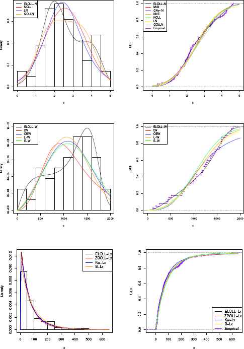
The fitted pdfs and the fitted cdfs for three data sets
A comparison of the proposed distributions with some of their sub-models using LR statistics is performed in Table 6. From Table 6, we can conclude that the ELOLL-N and ELOLL-W models yield a better fit to these data than the other two and three sub-models respectively. Also, there is no difference among the fits to the current data using the ELLOL-Lx, L-Lx and E-Lx models. In addition, these models provide a better representation of the data than the other sub-models based on the LR test at the 5% significance level.
| Model | Hypothesis | Test statistics | p-value |
| ELLOL-N vs L-N | H0:α=β=1, H1: H0 false | 6.9668 | 0.0307 |
| ELLOL-N vs E-N | H0:α=1, β=0, H1: H0 false | 7.3550 | 0.0253 |
| Model | |||
| ELLOL-W vs L-W | H0:α=β=1, H1: H0 false | 8.9952 | 0.01111 |
| ELLOL-W vs E-W | H0:α=1, β=0, H1: H0 false | 10.622 | 0.00494 |
| ELLOL-W vs | H0: β=0, H1: H0 false | 9.5252 | 0.00202 |
| Model | |||
| ELLOL-Lx vs L-Lx | H0: α=β=1, H1: H0 false | 4.7840 | 0.09144 |
| ELLOL-Lx vs E-Lx | H0: α=1, β=0, H1: H0 false | 4.7940 | 0.09099 |
| ELLOL-Lx vs OBLx | H0: β=0, H1: H0 false | 4.6560 | 0.03094 |
| ELLOL-Lx vs EL-Lx | H0: α=1, H1: H0 false | 4.7800 | 0.02879 |
| ELLOL-Lx vs LOLL-Lx | H0: β=1, H1: H0 false | 4.0060 | 0.04533 |
| ELLOL-Lx vs Lx | H0:α=θ=1, β=0, H1: H0 false | 10.7060 | 0.013426 |
LR statistics for three data sets
10. Conclusions
A new family of distributions called the exponential Lindley odd log-logistic G family is introduced and studied. The new family generalizes the Lindley-G family [9], Lehmann Type II-G family [19] and odd Burr-G family [4] as well as it introduces new distribution families such as exponential Lindley-G family and Lindley odd log-logistic-G family. We provide some mathematical properties of the new family including ordinary, generating function and order statistics. Characterizations based on truncated moments as well as in terms of the hazard function are presented. The maximum likelihood is used for estimating the model parameters. We give a simulation study for the maximum likelihood estimators by using the special member of new family. Finally, the usefulness of the family is illustrated by means of three real data sets. The new models provide consistently better fits than other competitive models for these data sets.
Appendix A.
Appendix B.
Theorem 1.
Let (Ω, ℱ, P) be a given probability space and let H = [d, e] be an interval for some d < e (d = −∞, e = ∞ might as well be allowed). Let X : Ω → H be a continuous random variable with the distribution function F and let q1 and q2 be two real functions defined on H such that
References
Cite this article
TY  - JOUR
AU  - Mustafa Ç. Korkmaz
AU  - Haitham M. Yousof
AU  - G. G. Hamedani
PY  - 2018
DA  - 2018/09/30
TI  - The Exponential Lindley Odd Log-Logistic-G Family: Properties, Characterizations and Applications
JO  - Journal of Statistical Theory and Applications
SP  - 554
EP  - 571
VL  - 17
IS  - 3
SN  - 2214-1766
UR  - https://doi.org/10.2991/jsta.2018.17.3.10
DO  - 10.2991/jsta.2018.17.3.10
ID  - Korkmaz2018
ER  -