
Chebyshev Polynomials, Rhodonea Curves and Pseudo-Chebyshev Functions. A Survey
- DOI
- 10.2991/gaf.k.200124.005How to use a DOI?
- Keywords
- Spirals; Grandi curves; pseudo-Chebyshev functions; recurrence relations; differential equations; orthogonality properties
- Abstract
In recent works, starting from the complex Bernoulli spiral and the Grandi roses, sets of irrational functions have been introduced and studied that extend to the fractional degree the polynomials of Chebyshev of the first, second, third and fourth kind. The functions thus obtained are therefore called pseudo-Chebyshev. This article presents a review of the elementary properties of these functions, with the aim of making the topic accessible to a wider audience of readers. The subject is presented as follows. In Section 2 a review of spiral curves is given. In Section 3 the main properties of the classical Chebyshev polynomials are recalled. The Grandi (Rhodonea) curves and possible extensions are introduced in Section 4, and a method for deriving new curves, changing cartesian into polar coordinates, is touched on. The possibility to consider the Grandi curves even for rational indexes allows to introduce in Section 5 the pseudo-Chebyshev functions, which are derived from the Chebyshev polynomials assuming rational values for their degree. The main properties of these functions are shown, including recursions and differential equations. In particular, the case of half-integer degree is examined in Section 6 since, in this case, the pseudo-Chebyshev functions verify even the orthogonality property. As a consequence, new system of irrational orthogonal functions are introduced.
- Copyright
- © 2020 The Authors. Published by Atlantis Press SARL
- Open Access
- This is an open access article distributed under the CC BY-NC 4.0 license (http://creativecommons.org/licenses/by-nc/4.0/).
1. INTRODUCTION
In writing an article on Growth and Shape, one cannot help but link the treatment to geometrical entities that translate those concepts into mathematical terms. They are the logarithmic spiral of Bernoulli, the curves of Lamé, the roses of Grandi, the lemniscate of Bernoulli and their generalizations.
The spiral has always been associated with growth phenomena, starting with that of the shell Nautilus widely studied in the book by Thompson [1] and in many subsequent works.
The Lamé’s curves have been generalized by J. Gielis in the 2D and 3D case in works [2,3] that have had wide international resonance [4–7].Grandi’s roses (also called Rhodoneas) and Bernoulli’s lemniscate have polar equations that lend themselves to being generalized, as is done here in Section 4.1. All these curves (or surfaces) of the plane (of space) lend themselves to creating mathematical forms that model natural forms [3].
In this article, starting from the spiral of Bernoulli, in the complex form, we make the obvious connection with the first and second kind Chebyshev polynomials, and with the roses of Grandi.
After that, having observed that roses also exist for rational index values, extensions of that polynomials are introduced in the case of fractional degree. Thus, irrational functions are found which are called pseudo-Chebyshev of first and second kind, because they continue to verify many of the properties of the corresponding Chebyshev polynomials.
Subsequently, using the links with Chebyshev polynomials of third and fourth kind and the good work [8], the pseudo-Chebyshev functions of third and fourth kind are also introduced and studied.
Particular importance is given, in Section 6, to the case of the half-integer degree, because, in this case, the pseudo-Chebyshev functions verify not only the corresponding recurrence relations and differential equations, but also the orthogonality properties, in the interval [−1, 1], with respect to the same weights of the classical polynomials.
In this survey we limited ourselves to considering only the most elementary properties of the pseudo-Chebyshev functions, which can be proven starting from trigonometric identities, that are known to secondary school students, so as to make the treatment usable to a wide audience. Moreover, the use of higher tools seems to be unessential in the context of this study, which deals with functions of elementary nature, connected in a simple way to trigonometric functions.
2. SPIRALS
The spiral symbol is found in every ancient culture, all over the world (see e.g. Figures 1, 2). The spiral is a sacred symbol, possibly reminding us the evolution of our life.
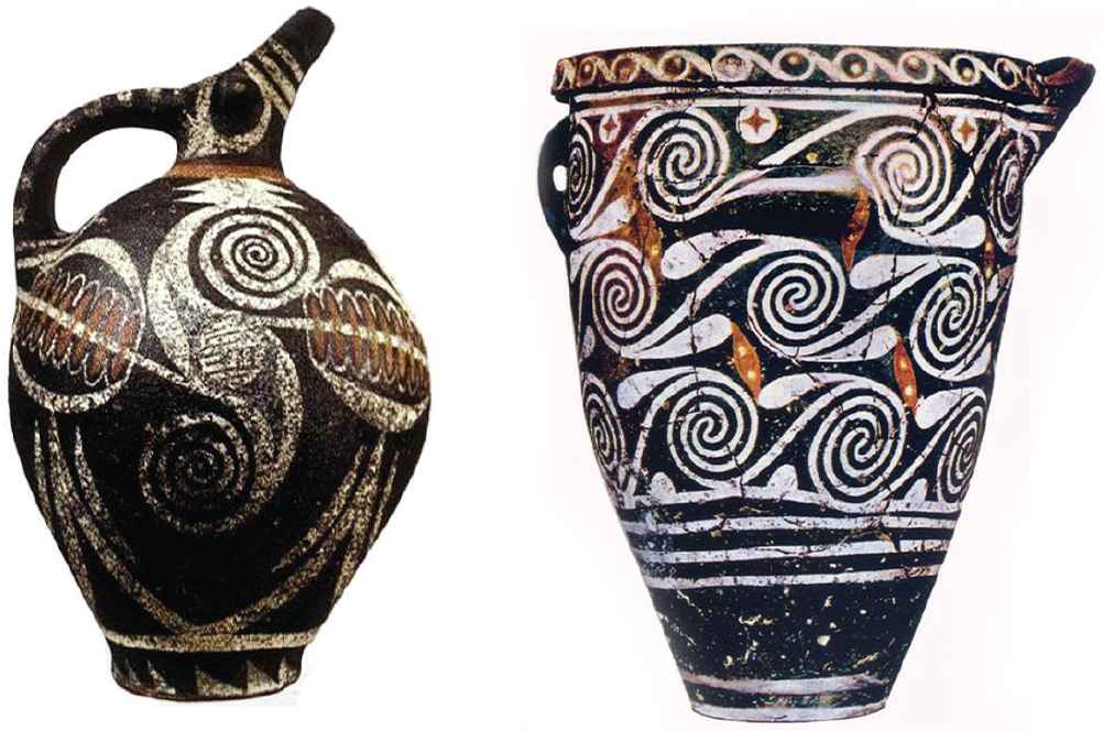
Ancient Crete island vases.
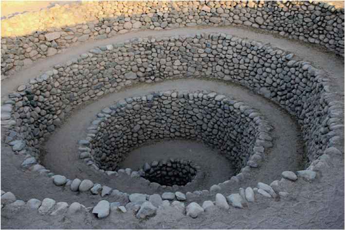
A a well of Nazca culture.
The first attempt to describe a spiral is due to Theodore of Cyrene, a mathematician from the school of Pythagoras, in the 5th century
By the mathematical point of view spirals are described by polar equations.
Many information on this subject can be found in Lockwood [9] and in Thompson [1], where applications to natural shapes (see e.g. Figure 3) are deeply analyzed. In a recent article [10] a Bernoulli spiral in complex form has been related to the Grandi (Rhodonea) curves and Chebyshev polynomials.
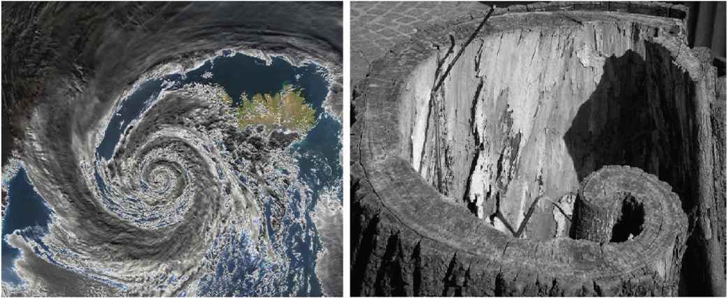
Spirals - natural shapes [29]
Connection with curvature can be found in Gielis et al. [11].
2.1. Archimedes vs Bernoulli Spiral
The Archimedes (Figure 4) spiral [12] (Figure 5) has the polar equation:
Archimedes (traditional) and his death by N. Barabino.
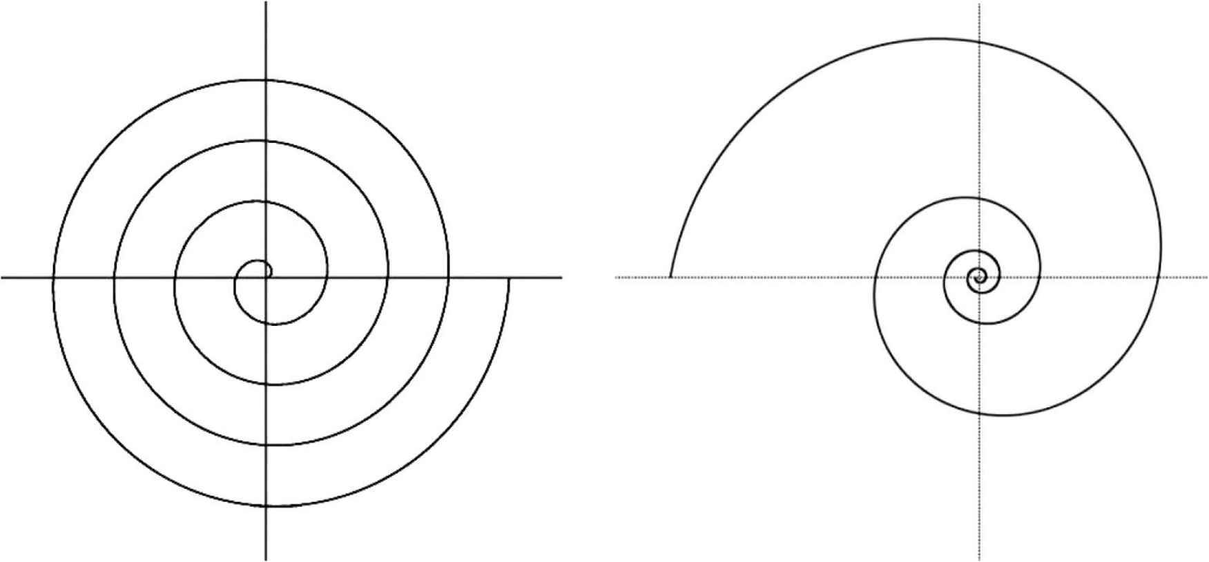
Archimedes vs Bernoulli spiral.
If θ > 0 the spiral turns counter-clockwise, if θ < 0 the spiral turns clockwise. Bernoulli’s (logarithmic) spiral [13] (Figure 5) has the polar equation
Varying the parameters a and b one gets different types of spirals.
The size of the spiral depends on a, while the term b controls the verse of rotation and how it is “narrow”.
Being a and b positive costants, there are some interesting cases. The most popular logarithmic spiral is the harmonic spiral, in which the distance between the spires is in harmonic progression, with ratio
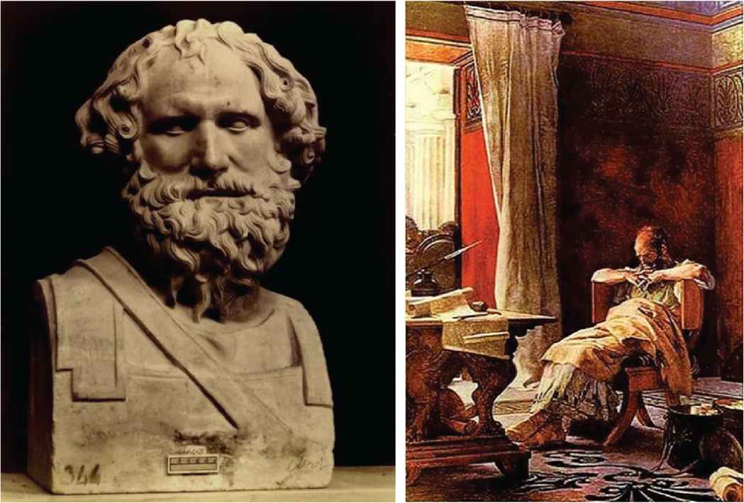
The logarithmic spiral was discovered by René Descartes in 1638, and studied by Jakob Bernoulli (1654–1705) (Figure 6).
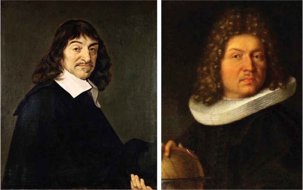
René Descartes by F. Hals and Jakob Bernoulli.
Pierre Varignon (1654–1722) called it spiral equiangular, because:
- 1.
There is a constant angle between the tangent at a given point and the polar radius passing through the same point.
- 2.
The inclination angle with respect to concentric circles centered at the origin is also constant.
It is a first example of a fractal. As it is written on J. Bernoulli’s tomb: Eadem Mutata Resurgo (but the spiral represented there is of Archimedes type).
2.2. Fermat Spiral, Fibonacci and Other Types of Spirals
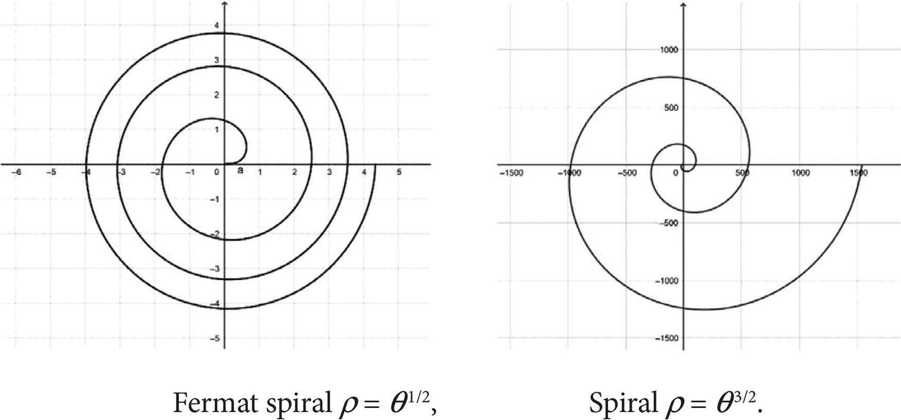
The Fermat (parabolic) spiral (Figure 7) has polar equation:
Fermat’s spiral suggests the possibility of introducing other kind of spiral graphs.
In fact there is a straightforward correspondence, between cartesian and polar systems of coordinates, which transforms y = f(x) functions of the (x, y) plane into polar curves ρ = f(θ) of the (ρ, θ) plane.
In this planar transformation, the Archimedes spiral ρ = aθ corresponds to the straight line y = ax, the Bernoulli spiral ρ = abθ to the exponential function y = abx, and the Fermat spiral to the parabolic function
Then, putting:
Notice that, if m > n, so that the exponent is >1, the coils of spiral are widening (Figure 7), while if m < n being the exponent <1, the coils of spiral are shrinking (as in Fermat’s case).
Other possibilities are:
- 1.
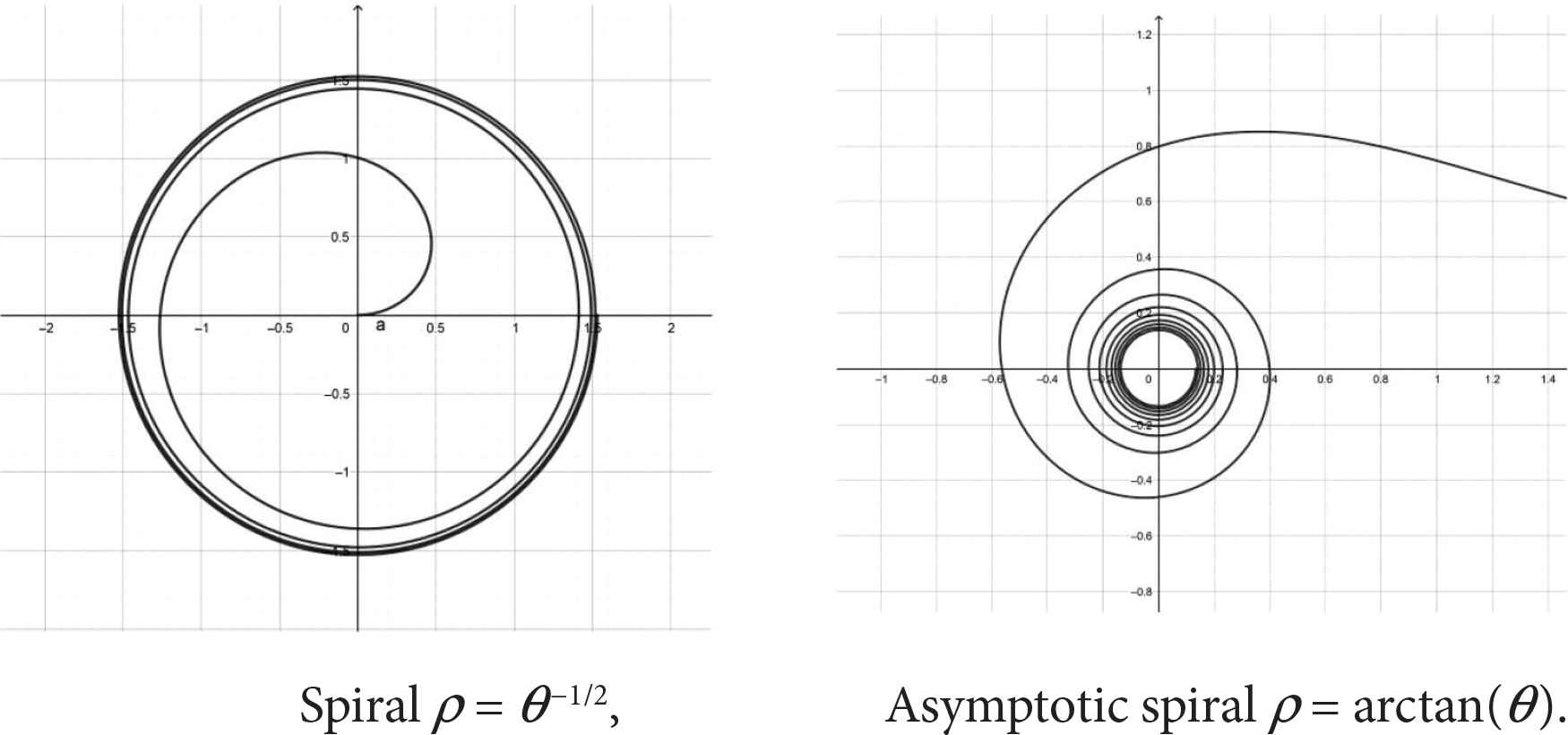
To assume θm/n with m/n < 0; in this case the coils are wrapped around the origin.
- 2.
To use a graph with horizontal asymptotes, in order to get an asymptotic spiral (Figure 8).
In what follows, we consider a “canonical form” of the Bernoulli spirals assuming a = 1, b = en, that is, the simplified polar equation:
2.3. The Complex Bernoulli Spiral
We now introduce the complex case, putting
Therefore, we have:
The curves with polar equation:
Curves with polar equation: ρ = sin(nθ) are equivalent to the preceding ones, up to a rotation of π/(2n) radians.
The Grandi roses display
- •
n petals, if n is odd.
- •
2n petals, if n is even.
By using Eq. (9) it is impossible to obtain, roses with 4n + 2 (n ∈ N ∪ {0};) petals.
Roses with 4n + 2 petals can be obtained by using the Bernoulli lemniscate and its extensions. More precisely,
- •
for n = 0, a two petals rose comes from the equation ρ = cos1/2(2 θ) (the Bernoulli lemniscate),
- •
for n ≥ 1, a 4n + 2 petals rose comes from the equation ρ = cos1/2[(4n + 2) θ].
Further very general extensions of the Bernoulli lemniscate are presented in Section 4.1.
3. CHEBYSHEV POLYNOMIALS
P. Butzer and F. Jongmans, in their biography of Chebyshev [14], assert that Pafnuty Lvovich Chebyshev (Figure 9) was the creator in St. Petersburg of the greatest Russian mathematical school before the revolution.
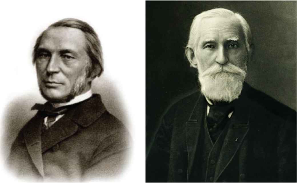
Pafnuty Lvovich Chebyshev (1821–1894).
Starting from the equations:
By comparing these equations with (10), we find:
Putting x = cost, in Eqs. (11) and (12) we find two polynomials, in the x variable, of degrees respectively n and n − 1, which are the first and second kind Chebyshev polynomials [15,16]:
3.1. Basic Properties of the Chebyshev Polynomials of the First Kind
The trigonometric equation
By using the initial values:
Note that:
- •
The leading coefficient of Tn(x) is equal to 2n−1.
- •
The polynomials T2n(x) are even functions and the T2n+1(x) are odd functions.
- •
- •
The n zeros of Tn(x) are real, distinct and internal to the interval [−1, 1].
More precisely, they are given by:
In fact, we have:
- •
The polynomials {Tn(x)} are orthogonal in the interval [−1, 1], with respect to the weight: (1 − x2)−1/2.
In fact, from the orthogonality of the cosine functions:
We furthermore have:
3.2. Basic Properties of the Chebyshev Polynomials of the Second Kind
In a similar way, the same recurrence relation holds for the second kind polynomials:
By using the initial values:
The polynomials {Un(x)} are orthogonal in the interval [−1, 1], with respect to the weight: (1 − x2)1/2:
We furthermore have:
Connections with the polynomials of the first kind
The second kind Chebyshev polynomials play an important role in representing the powers of a 2 × 2 non singular matrix [17,18]. Extension of this polynomial family to the multivariate case has been considered for representing the powers of a r × r (r ≥ 3) non-singular matrix (see [18,19]).
Remark 3.1.
Chebyshev polynomials are a particular case of the Jacobi polynomials
Therefore, properties of the Chebyshev polynomials could be deduced in a more general framework of the hypergeometric functions. However, in this approach the connection with trigonomeric function disappears. In this article, dealing with elementary functions, we use only elementary methods, in order to make the topic accessible to a wider audience of readers. In such a way, we avoid to shoot flies with cannons.
Remark 3.2.
In connection with interpolation and quadrature problems, another couple of Chebyshev polynomials have been considered. They correspond to different choices of weights:
These were called by Gautschi [20] the third and fourth kind Chebyshev polynomials, and will be considered in what follows.
3.3. Basic Properties of the Chebyshev Polynomials of Third and Fourth Kind
The third and fourth kind Chebyshev polynomials have been studied and applied by several scholars (see e.g. [8,21]), because they are useful in quadrature rules, when the singularities occur only at one of the end points (+1 or −1) (see [22]). Furthermore, recently they have been applied in Numerical Analysis for solving high odd-order boundary value problems with homogeneous or nonhomogeneous boundary conditions [21].
The third and fourth kind Chebyshev polynomials are defined in [−1, 1] as follows:
Since Wn(x) = (−1)nVn(−x), as it can be see by their graphs (Figures 10 and 11), the third and fourth kind Chebyshev polynomials are essentially the same polynomial set, but interchanging the ends of the interval [−1, 1].
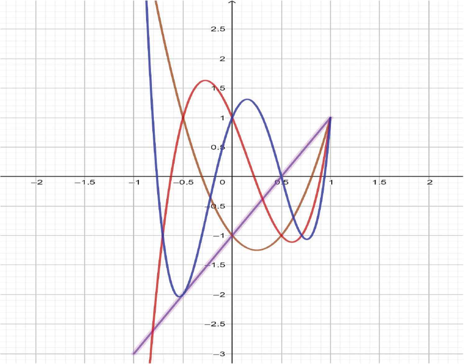
Vk(x), k = 1, 2, 3, 4. 1. violet, 2. brown, 3. red, 4. blue
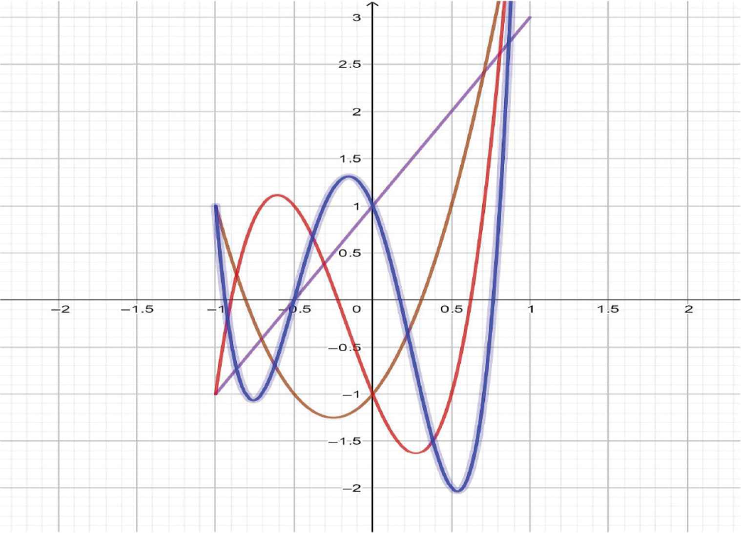
Wk(x), k = 1, 2, 3, 4. 1. violet, 2. brown, 3. red, 4. blue.
The orthogonality properties hold [8]:
One of the explicit advantages of Chebyshev polynomials of third and fourth kind is to estimate some definite integrals as
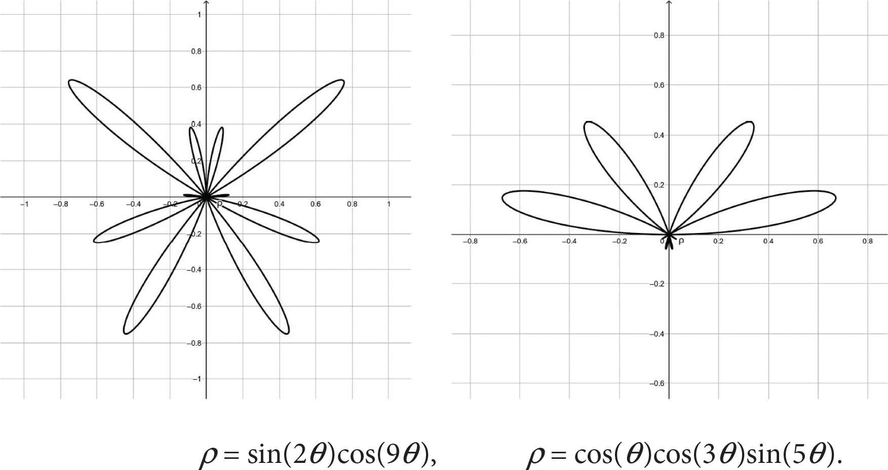
4. THE GRANDI (RHODONEA) CURVES
A few graphs of Rhodonea curves are shown in Figures 13–14.
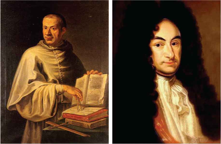
G. G. Grandi and G. W. Leibniz.

Rhodonea
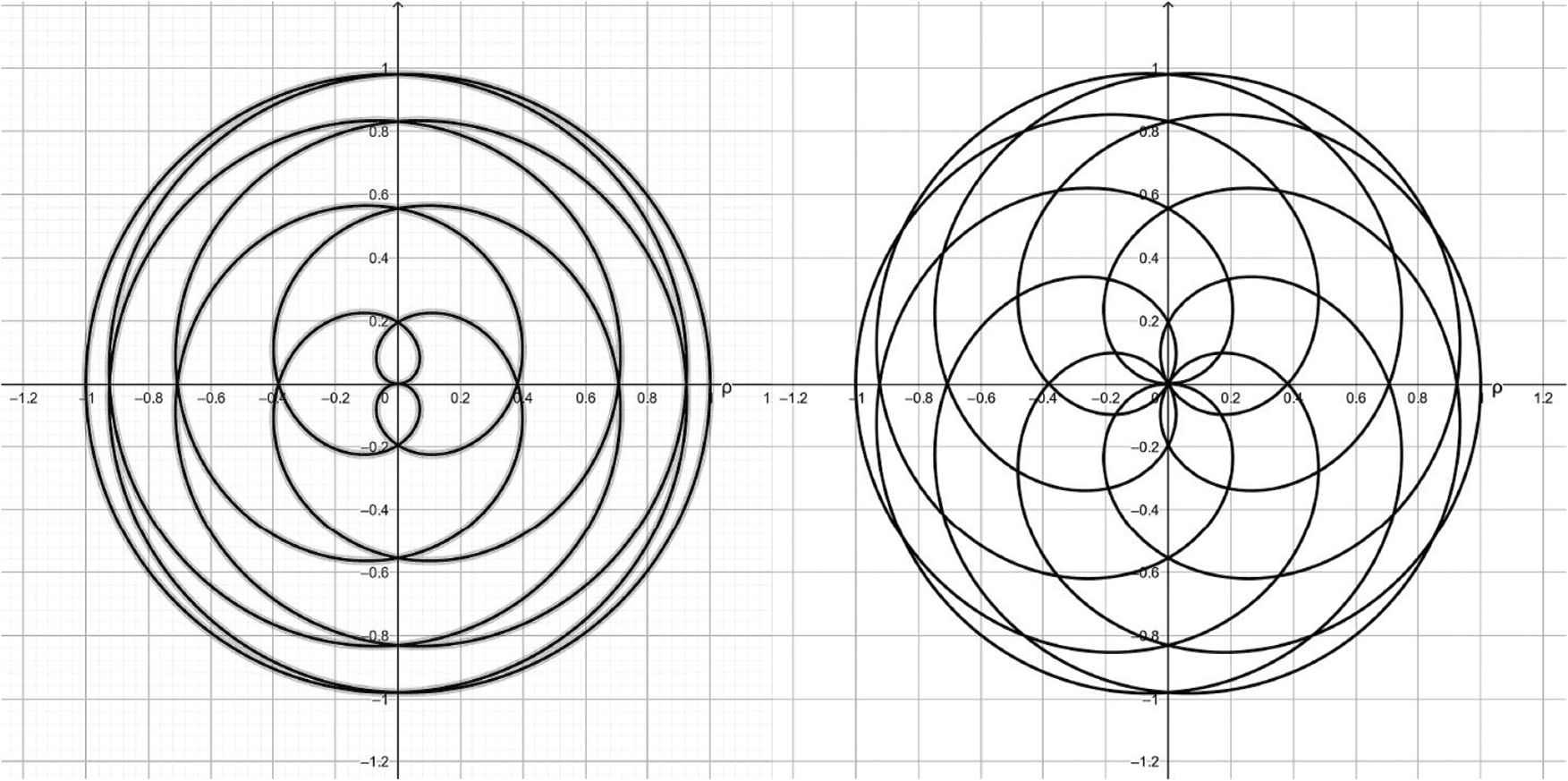
Rodoneas
4.1. Cartesian vs Polar Coordinates
The study of curves is of great importance for the modelling of natural objects and has attracted many scholars [9,23]. In particular, the so-called superformula by Gielis [2,3,5] has made it possible to construct the most diverse figures by varying a few parameters (see also [4,6,24]).
By exploiting the correspondence, mentioned in Section 2.2, between curves in the cartesian or polar form, we can find further graphs both of symmetric and asymmetric type.
In what follows we show some symmetric graphs, which does not coincide with the shapes of Grandi curves, and several others which are not symmetric. These graphs generalize in a wide way both the Grandi curves and the Bernoulli lemniscate recalled in Section 2.3.
To this aim, we consider first circular functions of the type:
The corresponding polar curves are:
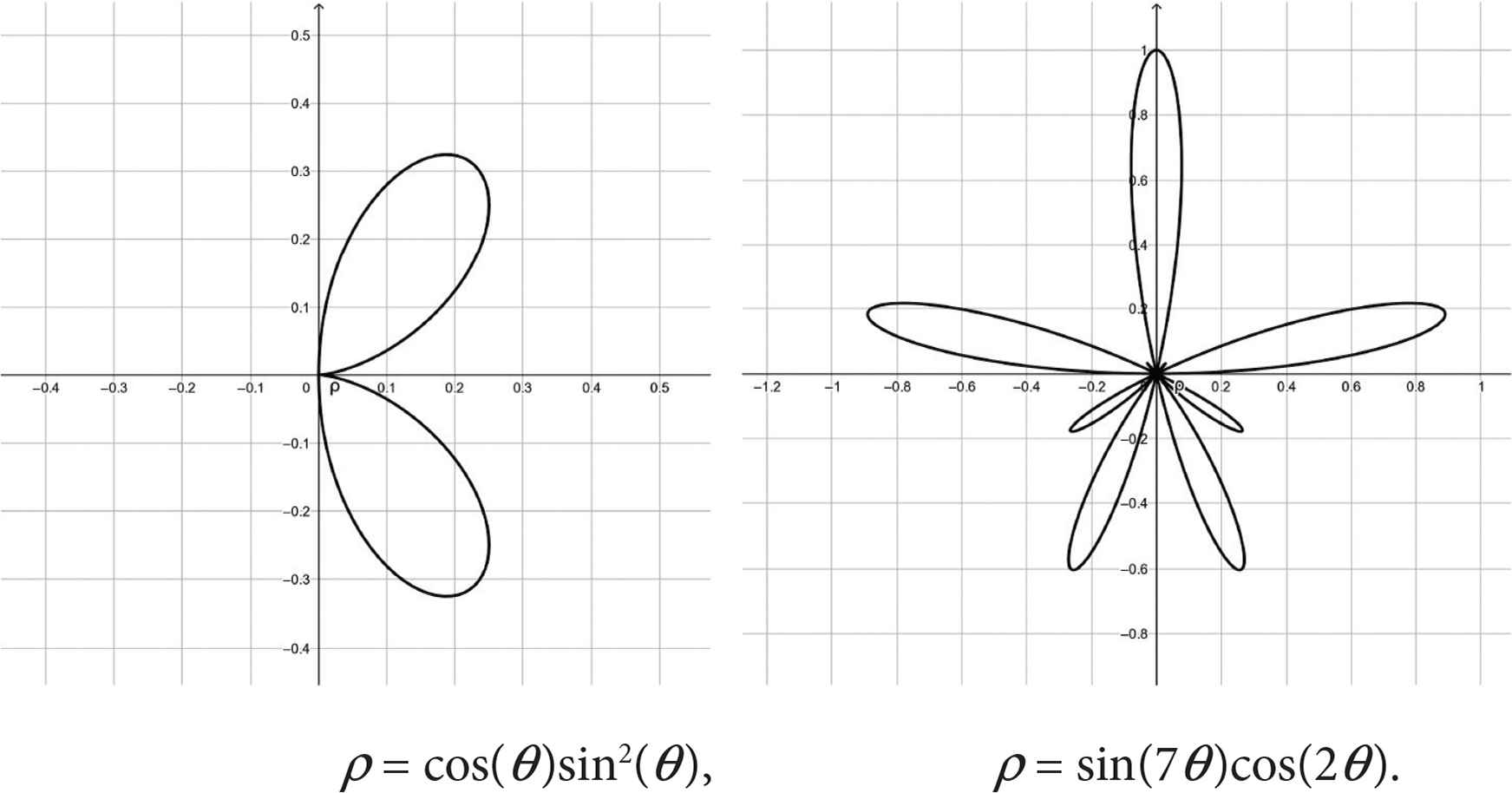
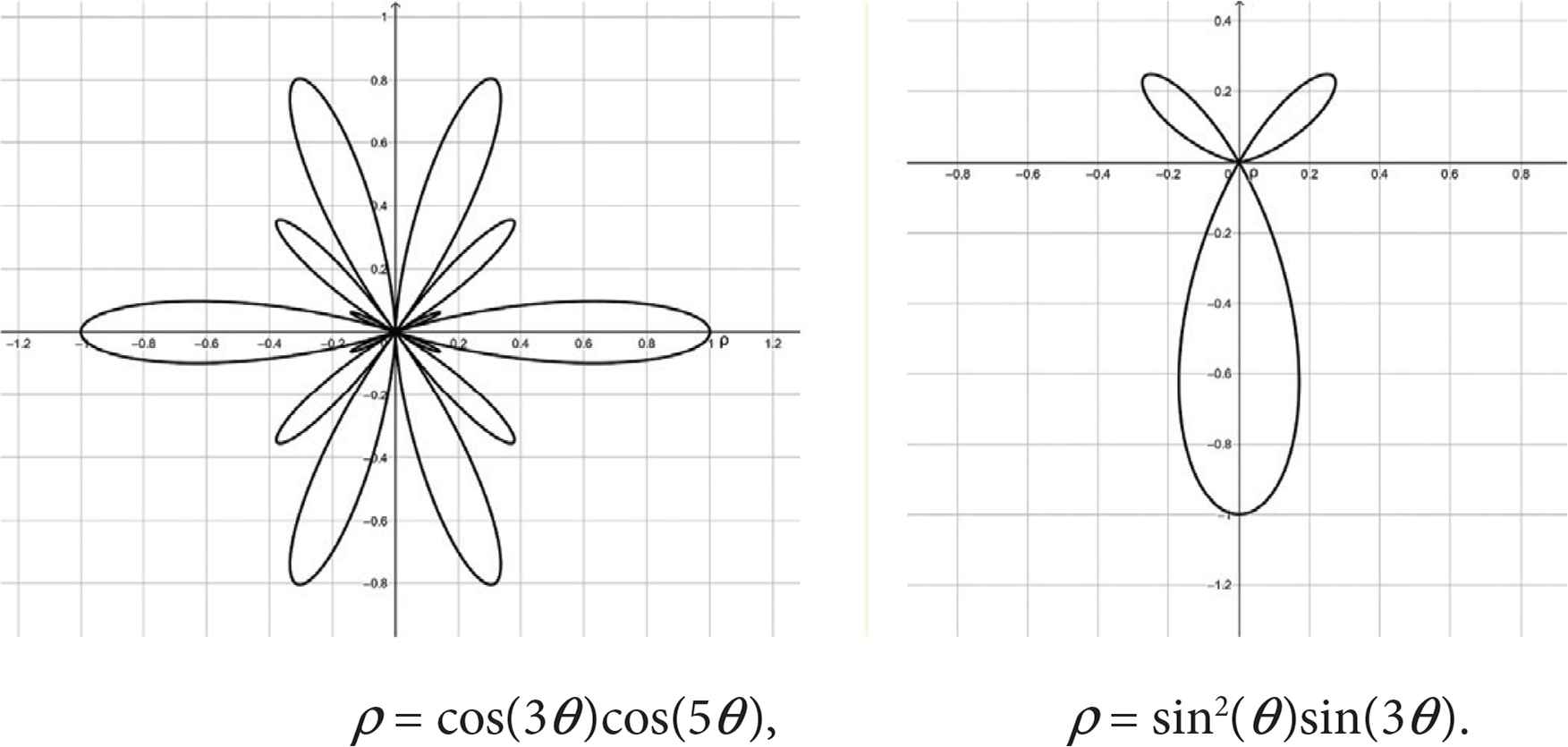
Of course we have more examples by changing sine by cosine or increasing the number of sine/cosine factors in the above trigonometric products.
The curves obtained in this way can be interpreted as a generalization of the Grandi roses.
A first example of this kind of figures can be found in Thompson [1] (Figure 504, page 1047), where the polar equation ρ = sin(θ/2)sin(nθ) can be found.
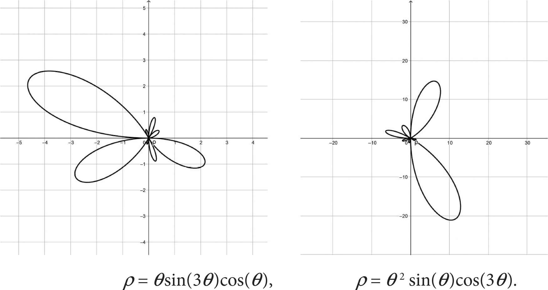
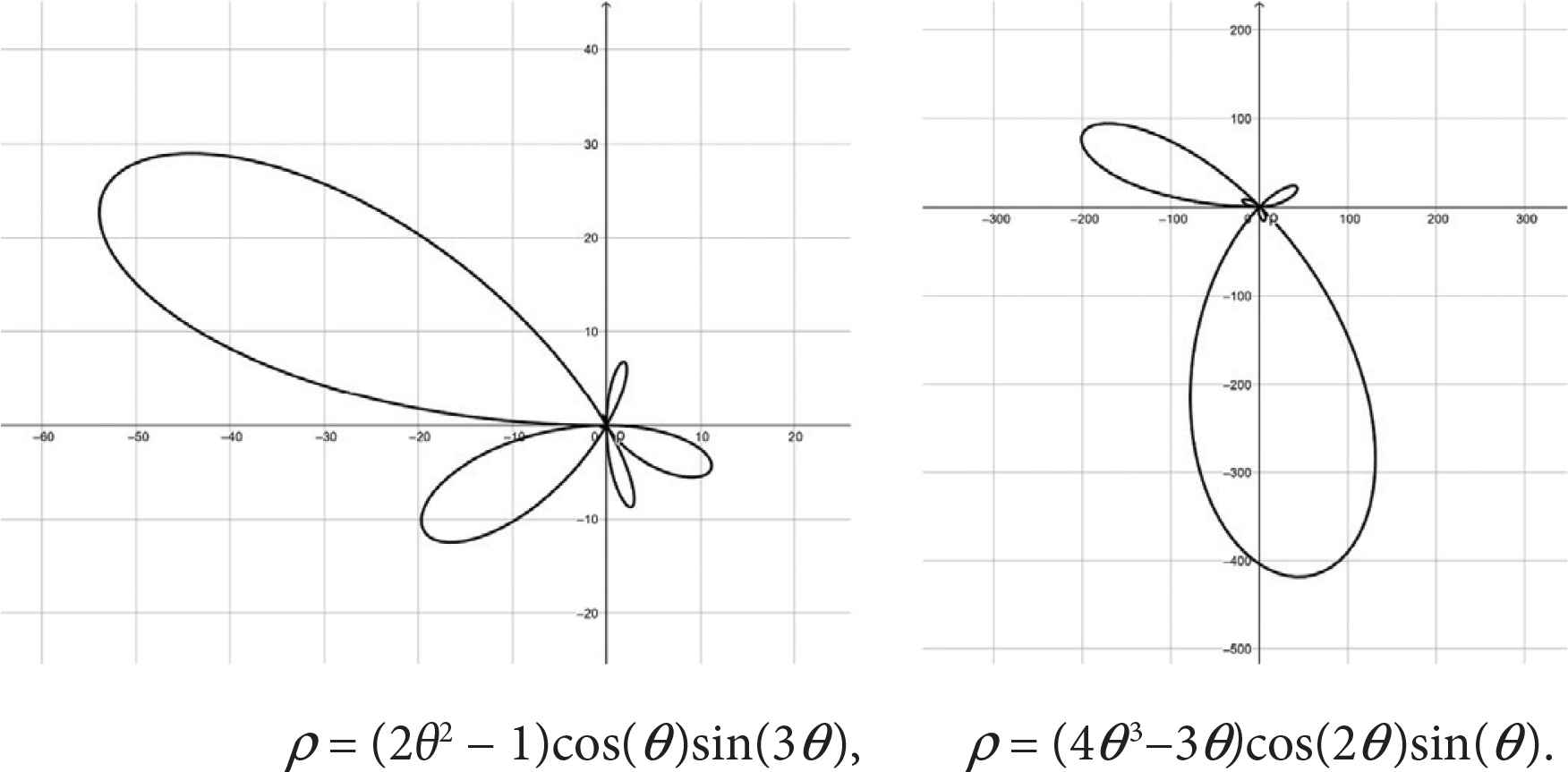
A infinite number of non-symmetric possibilities (generalizing in particular the Bernoulli lemniscate), are obtained by starting from the above circular functions multiplied by powers of the x variable (of polynomials Pq(x) of degree q), and taking positive rational numbers for the parameters m, n:
The graphic results obtained in these cases recall the inflatable balloons of children’s games. Note that in this case, the resulting curve may depend on the considered interval.
A few examples of this type are shown in Figures 18–22.
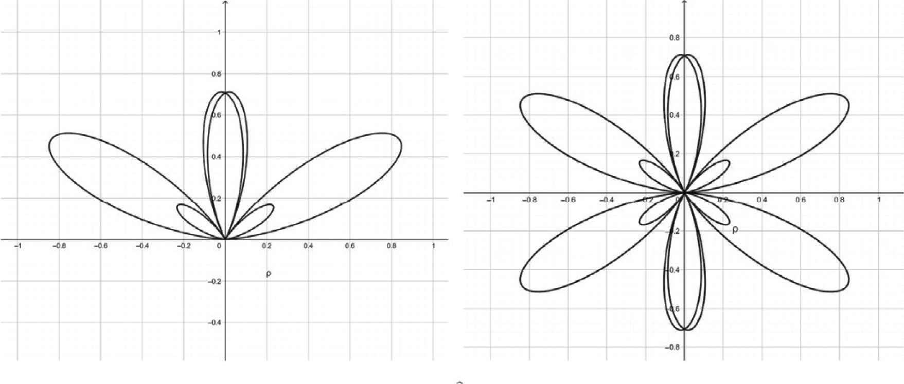
ρ = cos(θ/2)sin2(3θ) in [0, 2π] & in [0, 4π].
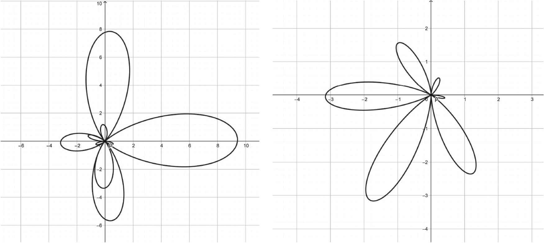
ρ = θ sin(θ/2)cos2(2θ) & ρ = θ sin(θ/2)cos2(3θ) in [0, 2π].
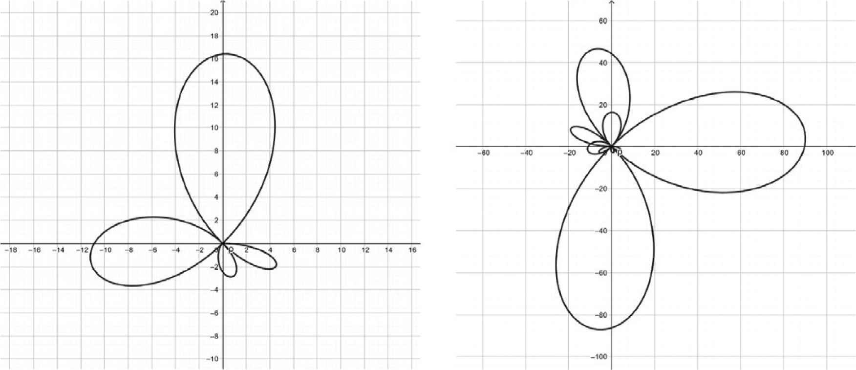
ρ = (θ2 + 1)sin(θ/2)cos(2θ) in [0, 2π] & in [0, 4π].
5. PSEUDO-CHEBYSHEV FUNCTIONS OF THE FIRST, SECOND, THIRD, FOURTH KIND
5.1. Basic properties of the First and Second Kind
We put, by definition:
Note that definitions (25) and (26) hold even for negative indexes, that is for p/q < 0, according to the parity properties of the trigonometric functions.
5.2. Pseudo-Chebyshev Functions of the First Kind
The following theorems hold:
Theorem 5.1.
The pseudo-Chebyshev functions Tp/q(x) satisfy the recurrence relation
Proof - Write Eq. (27) in the form:
Theorem 5.2.
The first kind pseudo-Chebyshev functions Tp/q(x) satisfy the differential equation:
Proof - Note that
5.3. Pseudo-Chebyshev Functions of the Second Kind
The following theorems hold:
Theorem 5.3.
The pseudo-Chebyshev functions
Proof - Write Eq. (29) in the form:
Theorem 5.4.
The pseudo-Chebyshev functions
The proof is obtained in a similar way to that of the first kind functions.
5.4. Basic Relations of the Pseudo-Chebyshev Functions of Third and Fourth Kind
According to Eq. (24), we put by definition:
Theorem 5.5.
The third and fourth kind pseudo-Chebyshev functions are related to the 1st and 2nd kind ones by the equations:
Proof - It is sufficient to use the addition formulas for the cosine and sine functions.
Therefore, we can derive the equations:
5.5. Some General Formulas
By using cosine addition formulas, putting:
5.5.1. Particular results
Combining the above equations, we find:
5.6. Links with the Pseudo-Chebyshev Functions
Actually, the definitions of the third and fourth kind Chebyshev polynomials are as follows:
Therefore, we find the equations:
6. THE CASE OF HALF-INTEGER DEGREE
In what follows, we consider the case of the half-integer degree, which seems to be the most interesting one, since the resulting pseudo-Chebyshev functions satisfy the orthogonality properties in the interval [−1, 1] with respect to the same weights of the corresponding Chebyshev polynomials [25].
Definition: Let, for any integer k:
Note that the above definition holds even for k + 1/2 < 0, taking into account the parity properties of the circular functions.
The pseudo-Chebyshev functions Tk+1/2 (x), Uk−1/2 (x), Vk+1/2 (x) and Wk+1/2 (x) can be represented, in terms of the third and fourth kind Chebyshev polynomials as follows:
We will show that, in the case of half-integer degree, the pseudo-Chebyshev functions satisfy not only the recurrence relations and differential equations analogues to the classical ones, but even the orthogonality properties.
6.1. Orthogonality of the Tk+1/2 (x) and Uk+1/2 (x) Functions
A few graphs of the
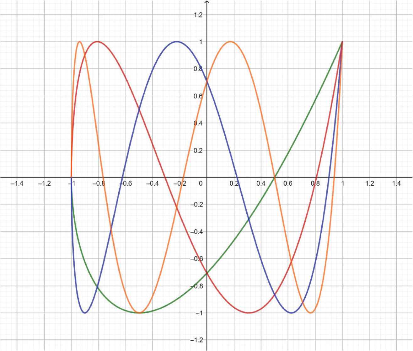
Tk+1/2 (x), k = 1, 2, 3, 4. 1. green, 2. red, 3. blue, 4. orange.
Theorem 6.1.
The pseudo-Chebyshev functions Tk+1/2 (x) satisfy the orthogonality property:
A few graphs of the Uk+1/2 functions are shown in Figure 24.
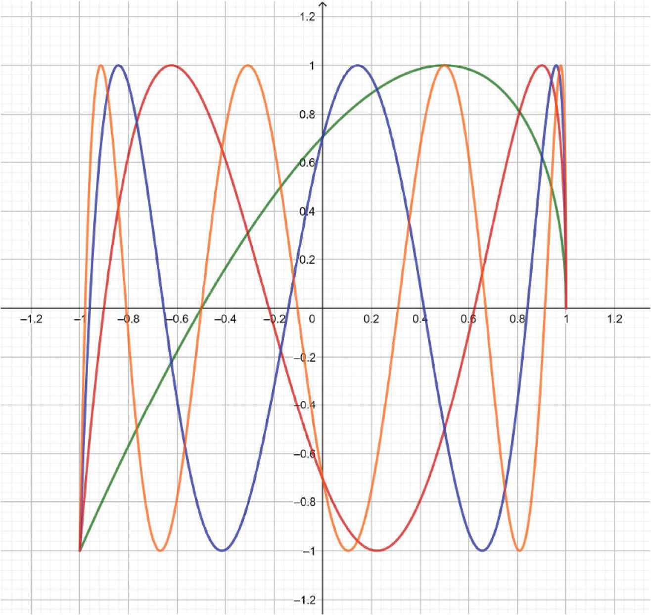
Uk+1/2 (x), k = 1, 2, 3, 4. 1. green; 2. red; 3. blue; 4. orange.
Theorem 6.2.
The pseudo-Chebyshev functions
Proof - We prove only Theorem 6.1, since the proof of Theorem 6.2 is similar.
From the Werner formulas, we have:
6.2. The Third and Fourth Kind Pseudo-Chebyshev Functions
The results of this section are based on the excellent survey by Aghigh et al. [8]. By using that article, it is possible to derive, in an almost trivial way, the links among the pseudo-Chebyshev functions and the third and fourth kind Chebyshev polynomials.
We recall here only the principal properties, without proofs. Proofs and other properties are reported in Cesarano et al. [27]. In Figures 25 and 26, we show the graphs of the first few third and fourth kind pseudo-Chebyshev functions.
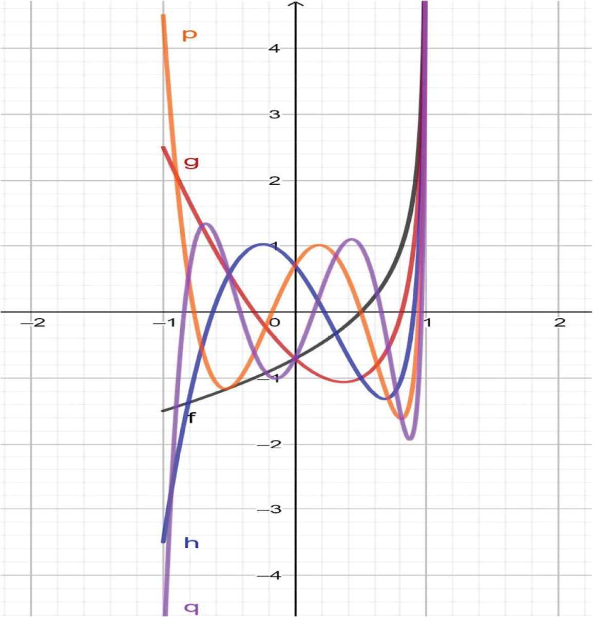
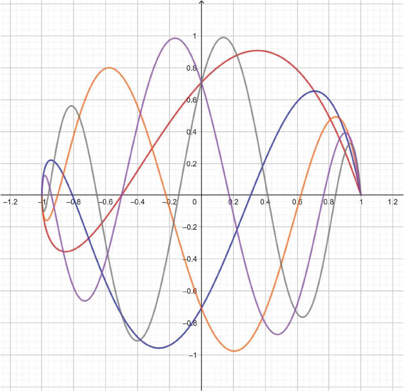
Vk+1/2 (x), k = 1, 2, 3, 4, 5. 1. grey, 2. red, 3. blue, 4. orange, 5. violet.
Wk+1/2 (x), k = 1, 2, 3, 4, 5. 1. red, 2. blue, 3. orange, 4. violet, 5. grey.
6.3. The Third Kind Pseudo-Chebyshev Vk+1/2
The third kind pseudo-Chebyshev functions satisfy the recurrence relation:
Theorem 6.3.
The pseudo-Chebyshev functions Vk+1/2(x) verify the differential equation:
The orthogonality property holds:
6.4. The Fourth Kind Pseudo- Chebyshev Wk+1/2
The fourth kind pseudo-Chebyshev functions satisfy the recurrence relation:
Theorem 6.4.
The pseudo-Chebyshev functions Wk+1/2 (x) verify the differential equation:
The orthogonality property holds:
6.5. Explicit Forms
Theorem 6.5.
It is possible to represent explicitly the pseudo-Chebyshev functions as follows:
6.6. Location of Zeros
By Eq. (48), the zeros of the pseudo-Chebyshev functions Tk+1/2(x) and Vk+1/2 (x) are given by
Remark 6.6.
More technical properties as the Hypergeometric representations and the Rodrigues-type formulas are reported in Cesarano et al. [26].
6.7. Links with First and Second Kind Chebyshev Polynomials
Theorem 6.7.
The pseudo-Chebyshev functions are connected with the first and second kind Chebyshev polynomials by means of the equations:
Proof - The results follow from the equations:
Remark 6.8.
Note that the first equation in (65), extends the known nesting property verified by the first kind Chebyshev polynomials:
This property, already considered in Brandi and Ricci [27] for the first kind pseudo-Chebyshev functions, actually holds in general, as a consequence of the definition Tk (x) = cos(k arccos(x)). Note that this composition identity even holds for the first kind Chebyshev polynomials in several variables, as it was proven in Ricci [28].
7. CONCLUSION
The growth of living organisms is often described by the Bernoulli’s logarithmic spiral, which is one of the first examples of fractals. The study of natural forms (see e.g. Bini et al. [29]) is commonly associated with mathematical entities like extensions of Lamé’s curves, Grandi’s roses, Bernoulli’s lemniscate, etc.
In this article, it has been shown that innumerable plane forms can be described by means of polar equations that extend some of the above mentioned geometrical entities. Moreover, the consideration of Grandi’s roses in the case of fractional indexes gives rise, in a natural way, to mathematical functions that generalize to the case of fractional degree the classical Chebyshev polynomials. The resulting functions, called of pseudo-Chebyshev type, verify many properties of the corresponding polynomials and, in the case of half-integer degree, also the orthogonality properties.
REFERENCES
Cite this article
TY  - JOUR
AU  - Paolo Emilio Ricci
PY  - 2020
DA  - 2020/02/23
TI  - Chebyshev Polynomials, Rhodonea Curves and Pseudo-Chebyshev Functions. A Survey
JO  - Growth and Form
SP  - 20
EP  - 32
VL  - 1
IS  - 1
SN  - 2589-8426
UR  - https://doi.org/10.2991/gaf.k.200124.005
DO  - 10.2991/gaf.k.200124.005
ID  - Ricci2020
ER  -