
Constructing Novel Operational Laws and Information Measures for Proportional Hesitant Fuzzy Linguistic Term Sets with Extension to PHFL-VIKOR for Group Decision Making
- DOI
- 10.2991/ijcis.d.190902.001How to use a DOI?
- Keywords
- Proportional hesitant fuzzy linguistic term set (PHFLTS); Comprehensive weighting model; Proportional hesitant fuzzy linguistic cosine similarity measure; Proportional hesitant fuzzy linguistic entropy measure; Multi-attribute group decision making (MAGDM); Extended PHFL-VKIOR method
- Abstract
To obtain reliable results in a qualitative multi-attribute group decision-making (MAGDM) problem, how to retain the evaluation information as much as possible and how to determine the reasonable weights of experts and attributes are two important issues. Proportional hesitant fuzzy linguistic term set (PHFLTS) is beneficial for retaining evaluation information as it would consider the linguistic terms and corresponding proportional information simultaneously. However, PHFLTS is a relatively new concept. Some novel manipulations, such as comparison, arithmetic operations, aggregation operators, and cosine similarity and distance measures are defined in this study with the purpose of improving the completeness and applicability of PHFLTS. Furthermore, cosine similarity measure-based weight determination model and entropy measure-based weight determination model under proportional hesitant fuzzy linguistic (PHFL) environment are constructed to derive the objective weights of experts and those of attributes as well. Subsequently, an integrated weighting model is proposed to determine the comprehensive weights of experts and attributes. Based on the defined operational laws for PHFLTS and comprehensive weighting model, two MAGDM methods, PHFL aggregation operator-based method and extended PHFL-VIKOR method, are developed to deal with MAGDM problems with PHFL information. To demonstrate the applicability, efficiency, and advantages of the proposed MAGDM methods, an illustrative example and a comparison example are provided.
- Copyright
- © 2019 The Authors. Published by Atlantis Press SARL.
- Open Access
- This is an open access article distributed under the CC BY-NC 4.0 license (http://creativecommons.org/licenses/by-nc/4.0/).
1. INTRODUCTION
“Decision-making” involves in almost all aspects of nearly every activity of our daily life. It is a cognitive process in which decision makers (DMs) make a choice among a set of alternatives in regard to certain criteria. As the criteria to which a decision is based on are multifaceted, the term of “multi-attribute decision making” (MADM) is therefore commonly used. Moreover, the increasing complexity of the decision-making environment makes more and more situations call for decisions to be made by a group of DMs so that a wider range of perspectives would be taken into consideration. Multi-attribute group decision-making (MAGDM) is growingly important but encounters two operation problems for coming up with reliable decisions. The first problem is how to retain the initial evaluation information and the second problem is how to determine the weights for the attributes and experts, which have direct influences on the final decision results, reasonably. Research in seeking ways for solving these two problems with MAGDM is of paramount importance.
To solve the first problem, the uncertainty and ambiguity of the evaluation information have to be taken into account. In fact, uncertainty and ambiguity are two prominent features of modern decision-making because of the dynamicity and complexity of the environment as well as the limited knowledge and cognition of DMs. Hesitant fuzzy linguistic approach [1], which based on hesitant fuzzy sets (HFSs) [2] and fuzzy linguistic term sets [3], has exhibited powerful capability in dealing with this situation. HFSs allow the DMs to offer more than one evaluation value on the alternatives to represent their hesitancy during an evaluation process, while fuzzy linguistic approach and computing with words [4–6] provide many linguistic terms and corresponding operations, which are closed to people's thoughts and cognition, for facilitating DMs to express their ideas and opinions [7]. Hesitant fuzzy linguistic term set (HFLTS), which was put forward by Rodríguez et al. [1], is the major tool for operating the hesitant fuzzy linguistic approach. In recent years, much research on studying HFLTS has been done because of its effectiveness. Wang [8] proposed extended HFLTSs (EHFLTSs) to release the consecutive constraint on linguistic terms used in HFLTSs. However, for both HFLTs and EHFLTs, information loss could easily be resulted as no proportional information is included in each linguistic term. To overcome this shortcoming, Zhang et al. [9] proposed linguistic distribution assessment of HFLTSs. It is a concept of which a DM was asked to assign subjective proportional information for his/her linguistic terms. Based on the work of Zhang et al. [9], Wu and Xu [10] proposed a possibility distribution of HFLTSs (PD-HFLTSs), in which the linguistic terms carry an equal possibility. More improved and enhanced methods [11–13] related to PD-HFLTSs have also been developed. Similarly, Chen et al. [14] proposed proportional hesitant fuzzy linguistic term sets (PHFLTSs) for group decision-making situations. The proportion is derived from statistical analysis of linguistic terms provided by DMs. The resultant decision derived by using PHFLTS would be of higher accuracy and reliability because the way of obtaining proportional information is objective and precise. For this reason, PHFLTS was adopted as the study subject of this research. Chen et al. [14] lay down some basic operational laws for PHFLTSs, including negation, union, intersection, comparison, and aggregation. However, no arithmetic operations, distance measures, and similarity measures were addressed in their study. Moreover, the complexity of their defined operations has limited practical application. To fill these gaps, some novel manipulations, such as comparison, arithmetical operation, cosine similarity and distance measures, and entropy measures for PHFLTSs are going to be defined in this paper to improve the availability and to decrease the computation complexity. On the whole, this study would help improve PHFLTS in theory and facilitate its practical application.
To consider the second problem aforementioned, the weights of experts and attributes would greatly affect the resultant decision. As the weights of experts are usually integrated into the weights of attributes, imprecision, if any, would be amplified. It implies that expert weights and attribute weights should be considered simultaneously. However, existing studies do not consider these two factors objectively and simultaneously. Pang et al. [15] constructed an adaptive consensus model to determine the optimal experts’ weights but those of attributes were subjectively given. Yu et al. [16] defined an extended TODIM method based on unbalanced HFLTSs with both the weights of experts and attributes were assigned by subjective determination. Wu et al. [17] proposed two MAGDM methods, VIKOR and TOPSIS, based on PD-HFLTSs. In these two methods, all experts carry the same weight whilst those of attributes were subjectively provided by the experts. Wang et al. [18] grouped experts into different importance levels by using linguistic variables and then determined the cluster weight for each small group. However, the weights of attributes had not been considered. To our best knowledge, there is still no existing research focused on the weight determination of experts and attributes simultaneously and comprehensively. To fill this gap, this study is going to present a comprehensive weighting model for determining the weights of experts and attributes both simultaneously and comprehensively. The objective weights of experts and attributes are first determined by basing on the proposed cosine similarity measure and entropy measure for PHFLTSs respectively. The obtained objective weights are then integrated with the subjective weights derived by AHP method to generate the comprehensive weights. The resultant weights, therefore, contain both the subjective preferences of DMs and the objective information embodied in the evaluation data.
The selection of decision-making approach is another important issue in MAGDM problems. A variety of MAGDM methods have been developed and applied for different decision environments for examples, the TOPSIS method [19–23], the PROMETHEE method [24,25], the TODIM method [16,26,27], and the VIKOR method [28,29]. Among these mentioned methods, VIKOR is an ideal point-based MAGDM method for dealing with discrete decision problems with non-commensurable and conflicting criteria [30]. The VIKOR method would lead to more reasonable decision results as it derives compromise solution(s) by maximizing group utilities and minimizing individual regrets, and, considers the subjective preference of DMs as well. In this paper, an extended version of VIKOR under PHFL environment (PHFL-VIKOR) based on the defined operational laws and cosine distance measure for PHFLTSs is proposed.
The remainder of this paper is organized as follows. Section 2 discusses several crucial concepts that related to our study. Section 3 defines some novel manipulations for PHFLTSs, including comparison method, arithmetical operational laws and corresponding properties, aggregation operators, and, cosine similarity and distance measures. Section 4 constructs an integrated weighting model for determining the comprehensive weights of experts and attributes in MAGDM problems with PHFL information. Section 5 provides two MAGDM methods, PHFL aggregation operator-based method and extended PHFL-VIKOR method, with detail steps. In Section 6, besides a numerical example is provided for illustrating the applicability and efficiency of the proposed methods, the influence on the weights of experts and the weights of attributes on the decision results of the illustrated example is also discussed. There is also a comparison between the proposed approach and other methods so as to present the necessity of incorporating the proportional information into HFLTSs as well as determining reasonable weights of experts and attributes for obtaining reliable decision results. Furthermore, a sensitivity analysis demonstrating the influence of decision-making strategy, represented by a coefficient when calculating the comprehensive evaluation values, on the alternative ranking in the extended PHFL-VIKOR method, is presented. Last but not least, Section 7 concludes the paper with a brief summary and lays down suggestions and directions for future research.
2. PRELIMINARIES
This section mainly recalls several basic definitions, operations, and properties of linguistic term sets (LTSs), HFLTSs, EHFLTSs, PD-HFLTSs, and PHFLTSs that provide the ground for this research.
2.1. Linguistic Term Sets
The LTSs are the basis of fuzzy linguistic decision-making approach [3], in which the evaluation information is expressed in a qualitative manner. There are two kinds of commonly used linguistic scales. The first kind is the subscript-symmetric additive linguistic term set [31]
For the convenience of computation and information retention, Xu [33] extended the discrete LTS to a continuous form as
2.2. Hesitant Fuzzy Linguistic Term Sets
Rodríguez et al. [1] proposed the concept of HFLTSs based on HFSs [2] and fuzzy linguistic approach [3] to deal with the situation in which DMs are hesitant among multiple possible linguistic terms when evaluating an alternative with respect to certain attributes.
Definition 1.
[1] Let
Obviously, the linguistic terms in an HFLTS are required to be consecutive, while it may not always be satisfied in practical applications. Therefore, Wang [8] presented the concept of EHFLTS based on the definition of HFLTS.
2.3. Extended Hesitant Fuzzy Linguistic Term Sets
Definition 2.
[8] Let
Theorem 1.
[34] Construction axiom: the union of HFLTSs leads to EHFLTS.
The construction axiom demonstrates the relationship between HFLTSs and EHFLTS. Considering a GDM problem, in which the priorities of individuals are completely unknown. If the evaluation results of individuals are represented by HFLTSs, then the group evaluation results can be represented by EHFLTS through the combination of each HFLTS provided by individuals.
As HFLTSs and EHFLTSs only contain the linguistic terms but not any proportional information, there is a lack of expert support for each linguistic term under GDM environment. To deal with this problem, Zhang et al. [9] put forward the concept of linguistic distribution assessment of HFLTSs that containing support degrees or symbolic proportions corresponding to the linguistic terms.
Definition 3.
[9] Let
2.4. Possibility Distribution for HFLTSs
Based on the aforementioned work, Wu and Xu [10] proposed the concept of possibility distribution for HFLTSs (PD-HFLTSs) in which each element has an equal possibility indicating the support degree of an expert. PD-HFLTS is an important extension of HFLTSs. Let
Definition 4.
[10] Let
In Eq. (1),
The discrimination among different HFLTSs defined on the same
Definition 5.
[10] Let
When comparing two HFLTSs,
Definition 6.
[10] Let
2.5. Proportional Hesitant Fuzzy Linguistic Term Sets
Based on the relationship analysis of fuzzy linguistic approach, HFLTS, EHFLTS, linguistic distribution assessment of LTS, and PD-HFLTS, Chen et al. [14] proposed a novel linguistic representation model for considering the linguistic terms and the corresponding proportions simultaneously under GDM environment. Before providing the definition of PHFLTS, it is necessary to learn about the concepts of proportional linguistic pairs and ordered proportional linguistic pairs that would be used in the definition of PHFLTS.
Definition 7.
[14] Let
Definition 8.
[14] Let
Remark 1.
It is worth noting that the sum of
Let us first introduce two practical cases to explain the situations where the sum of
Case 1. Considering a problem of evaluating university faculty for tenure and promotion [35]. Ten experts (
Case 2. The background of the problem is same as Case 1; and, the sum of
The proposed proportion normalization method of this research is composed of the following four steps:
Step 1. Calculate the cardinality of each HFLTS provided by the corresponding expert.
Let
Step 2. Calculate the least common multiple (LCM) of all
Step 3. Calculate the multiple
Step 4. Calculate the proportion
Based on the proposed normalization method, the following calculation process would be displayed. For Case 1, First, obtain ten HFLTSs that denote the evaluation results corresponding to each expert, that is,
As PHFLTS is a newly proposed concept, a series of novel basic operational laws, a comparison method, and aggregation operators for PHFLTSs are proposed in this paper for making a significant improvement for the availability and efficiency of PHFLTS. Furthermore, the cosine similarity and distance measures for PHFLTSs from a geometric perspective to facilitate qualitative decision-making are also defined.
3. SOME NOVEL PROPOSITIONS FOR PHFLTSs
3.1. The Comparison between PHFLTSs
It is necessary to develop a comparison method for PHFLTSs for more effective use when ranking alternatives that represented by PHFLTSs. Not only linguistic terms but also proportional information is included in PHFLTSs. These two aspects should be simultaneously considered when comparing two PHFLTSs. In the previous studies of comparing HFLTSs, Rodríguez et al. [1] used the interval values to rank HFLTSs based on the concept of envelope. Zhang et al. [36] defined an expectation and a variance function to compare any two hesitant linguistic distributions (HLDs). Zhang et al. [9] proposed a comparison method for linguistic distribution assessment based on expectation value and the inaccuracy function. Wu and Xu [10] proposed an expectation and variance-based comparison method for PD-HFLTSs (Definitions 5 and 6). All these mentioned comparison methods have a characteristic in common when dealing with linguistic terms. They all used the subscript of linguistic terms directly based on the operational laws defined in Section 2.1. However, as Gou and Xu [37] pointed out, the subscript of the result linguistic terms may exceed the bounds of predefined linguistic term sets when using the subscripts directly in the computation process. To solve this problem, Gou et al. [38] proposed two equivalent transformation functions to achieve the goal of transformation between HFLTSs and HFSs.
Definition 9.
[38] Let
Inspired by the above two transformation functions, the expectation function of PHFLTSs is proposed by this research.
Definition 10.
Let
When comparing two PHFLTSs
Definition 11.
Let
For comparing two PHFLTSs,
3.2. Some Basic Operational Laws for PHFLTSs
Generally, the number of elements, that is, the proportional linguistic pairs, in different PHFLTSs are different. In order to make the operation easier, it is necessary to make the elements the same. The traditional way is to add the smallest linguistic term to the set with relatively small elements until they have the same number of linguistic terms. Moreover, the added linguistic terms are endowed with the proportion of zero. However, it may be unreasonable because it could result in information distortion. As previously stated, the operation of PHFLTSs have to consider the linguistic terms and proportional information simultaneously, while the added proportion, zero, could change the computation results. Therefore, an appropriate way for doing it is to adjust the PHFLTSs to having the same number of elements without increasing or decreasing any elements. Wu et al. [39] proposed an approach for adjusting the probabilistic linguistic terms (PLTs) of which the same set of proportion could be used, based on the idea that the linguistic terms having the same subscript can be combined or split by adjusting their probability. Considering the similarity between PHFLTs and PLTs and inspired by the method for dealing with PLTs, the specific adjustment process is presented as follows:
Definition 12.
Let
if
or if
if
or if
or if
or if
As the adjustment is based on the idea that the linguistic terms which have the same subscript can be integrated or split by adjusting their proportions, the linguistic terms, as well as their corresponding total proportions, are not changed in the adjusted PHFLTSs.
Any two PHFLTSs with different number of proportional linguistic pairs could be adjusted to have the same number of proportional linguistic pairs by using the above-mentioned adjustment method. Besides, both of the adjusted PHFLTSs are sharing the same proportional vector. Therefore, the following basic operational laws for PHFLTSs based on Definitions 9 and 12 are proposed.
Definition 13.
Let
As the proposed operational laws are based on the transformation function
Example 1.
Let
Theorem 2.
Let
The proof for Theorem 2 can refer to Appendix A
3.3. Two Aggregation Operators for PHFLTSs
Appropriate aggregation operators are beneficial to MAGDM. For better utilization of PHFLTSs in constructing decision-making approaches, the following two aggregation operators based on the defined operational laws are proposed.
Definition 14.
Let
Example 2.
Let
Definition 15.
Let
3.4. Cosine Similarity and Distance Measures for PHFLTSs
Cosine similarity, from the geometric perspective, is defined as the measure of the difference between two individuals using the cosine value of the angle between two non-zero vectors. Compared to traditional similarity and distance measures that defined from the algebraic perspective, cosine similarity pays more attention on the difference of the direction between two vectors, rather than distance or length. The cosine similarity and distance are more commonly used to distinguish the difference from the direction, rather than the absolute numerical value. Therefore, it uses the user's qualitative evaluation of the content to distinguish the similarity and the difference. Additionally, the cosine similarity measure is not affected by the indicator scale, therefore, it could effectively overcome the problem of non-uniform metrics of the users; in particular when the score trend of two users is the same but the numerical values are very different, the cosine similarity measure would more likely provide a better solution. For example, when two users provide the vector (3, 3) and (5, 5) respectively, the solution that given by algebraic distance is not so reasonable as the cosine similarity because they both carry the same cognition. The definition of cosine similarity is initially represented by the following.
Definition 16.
[41] Let
Due to the superiority and practicability of cosine similarity, it has been extended to fuzzy sets [42,43], intuitionistic fuzzy sets [44], and HFLTSs [44] in terms of theory. Accordingly, the cosine similarity and its extension have been widely applied in the field of text and pictures similarity computation, medical diagnosis, anomaly detection in web documents, and production prediction in petrochemical industries in terms of application. Inspired by the above ideas, the cosine similarity measure for PHFLTSs is proposed as follows:
Definition 17.
Let
Especially, we adopt the convention
It is obvious that the proposed cosine similarity for PHFLTSs satisfies the fundamental axioms given by Liao et al. [45], that is,
The proof can refer to Appendix B.
With reference to the relationship between distance measures and similarity measures proposed by Liao et al. [45], the cosine distance measure for PHFLTSs therefore could be obtained accordingly:
In consistent with the proposed cosine similarity, we also adopt the convention
The cosine distance measure obviously satisfies the axiom of distance measure, that is,
Based on the relationship between cosine distance and cosine similarity, it is obvious that the cosine distance exhibits the three axioms, too. However, the cosine distance measure is not a proper distance metric because it does not satisfy the property of triangle inequality and it violates the coincidence axiom. In order to repair the triangle inequality property without altering the order, it is necessary to transform into angular distance. That is,
4. COMPREHENSIVE WEIGHTING APPROACH UNDER PHFL ENVIRONMENT
In an MAGDM problem, reasonable determination for the weights of experts and attributes is an important issue as it would influence the accuracy and reliability of decision-making. In regard to this importance, a weighting approach for determining the comprehensive weights of experts and attributes in MAGDM with PHFL information is proposed. It is a comprehensive weighting approach that would simultaneously consider the subjective weights and the objective weights.
4.1. Problem Description
In a fuzzy linguistic MAGDM problem, the experts set is
4.2. Experts’ Objective Weights Determination Using Cosine Similarity for PHFLTSs
The individual evaluation results have to be similar to those of the group evaluation results for confirming the consistency. The smaller the similarity, the bigger the difference. Therefore, smaller weights should be assigned for those experts whose evaluation results are far from the group evaluation results. Based on this idea, a weighting approach, calculating the similarity between individuals and group according to the proposed cosine similarity measure for PHFLTSs, for determining the objective weights of experts is proposed.
Assuming that the evaluation results of
As previously stated, as experts with greater similarity would make more reliable evaluation, so larger weights should be assigned. The normalized similarity could be recognized as the objective weights of experts. Then,
Based on the subjective weights obtained by AHP and the objective weights obtained by the similarity measure, we could obtain the comprehensive weights of experts, using a simple linear weighting method.
4.3. Attributes’ Objective Weights Determination Based on Entropy Measure for PHFLTSs
Similar to the weights of experts, the weights of attributes would also impose a significant influence on the evaluation results of MAGDM problems. The method that widely used for determining the objective weights of attributes is the entropy method. In the following, an entropy measure for PHFLTSs that used to determine the objective weights of attributes is proposed. It is commonly believed that the attributes with smaller entropy should be assigned with greater weights. Liu et al. [46] proposed fuzzy entropy, hesitant entropy, and total entropy for PLTSs. As a result, a total of 144 different entropy measures were obtained from the combinations made between fuzzy entropy and hesitant entropy. Motivated by these ideas, an entropy measure for PHFLTSs is proposed as follows:
Definition 18.
Let
To obtain the objective weights of attributes using the above-proposed entropy measure method, it is necessary to first calculate the weighted evaluation matrix of attributes,
Then, compute the average entropy of each attribute under all alternatives as follows:
Finally, calculate the objective weights of attributes using the following formula.
Based on the subjective weights obtained by AHP and the objective weights obtained by the entropy measure, we could obtain the comprehensive weights of attributes using a simple linear weighting method as follows:
The comprehensive weights of experts and attributes that have been obtained is going to be used to obtain more reliable results in the subsequent decision-making process. The detailed process of the proposed comprehensive weighting model could be expressed as the following algorithm.
4.4. Algorithm to Obtain the Comprehensive Weights of Experts and Attributes
Step 1. Determine the subjective weights of experts and attributes by AHP method, and denote them as
Step 2. Based on the
Step 3. Determine the objective weights,
Step 4. Calculate the comprehensive weights,
Step 5. Re-generate the group evaluation matrix of alternatives under all attributes using the comprehensive weights,
Step 6. Determine the objective weights,
Step 7. Calculate the comprehensive weights,
5. TWO MAGDM METHODS UNDER PHFL ENVIRONMENT
In the following, two MAGDM methods under the PHFL environment are going to be proposed. The description of the decision-making problem is the same as the definition in Section 4.1.
5.1. PHFL Aggregation Operator-Based MAGDM Method
The specific process of the proposed MAGDM method based on the proposed PHFLWA operator is described as follows:
Step 1. Define the LTS and the specific meaning of each linguistic term used in the evaluation process. This step determined what linguistic terms the experts could use to provide their opinions on the alternatives with respect to the attributes based on their professional knowledge and social experience.
Step 2. Determine the subjective weights of experts and attributes using the AHP method.
Step 3. Generate the evaluation information matrix on each alternative with respect to each attribute given by each expert.
Step 4. Generate the group evaluation matrix of each alternative under each attribute, and, calculate the proportional information of each linguistic term in the group evaluation matrix using statistical analysis based on the subjective weights of experts and attributes.
Step 5. Obtain the individual evaluation results of each expert as well as the integrated group evaluation results of each alternative based on the single evaluation matrix provided by each expert.
Step 6. Determine the comprehensive weights of experts and attributes based on the proposed method in Section 4.2 and Section 4.3.
Step 6.1. Determine the objective weights of experts based on cosine similarity measure according to Eqs. (16) and (17).
Step 6.2. Determine the comprehensive weights of experts by integrating the subjective weights with the objective weights according to Eq. (18).
Step 6.3. Determine the objective weights of attributes based on the entropy measure according to Eqs. (20) and (21) with updated experts’ comprehensive weights.
Step 6.4. Determine the comprehensive weights of attributes by combining the subjective weight with the objective weights according to Eq. (22).
Step 7. Re-generate the group proportional hesitant fuzzy linguistic evaluation matrix based on the obtained comprehensive weights of experts and attributes using the proposed operations for PHFLTSs in Section 3.2 and Section 3.3.
Based on the determined comprehensive weights of experts
Step 8. Determine the ranking of all alternatives.
Based on the addition operational law of PHFLTSs proposed in Definition 13, the final score of each alternative
5.2. Extended VIKOR Method with PHFL Information
As mentioned in the introduction of this paper, VIKOR is an efficient and widely used method for ranking a set of alternatives, and many extensions of it have been studied. However, there is still no research conducted on VIKOR with PHFL information. In view of this, an extended version of VIKOR, which is denoted as PHFL-VIKOR, under PHFL environment is proposed. The detail process is depicted as follows:
Step1 ~ Step 7. These steps are the same as Step 1 to Step 7 in Method 1.
Step 8. Determine the positive value,
Particularly, when comparing
Step 9. Calculate the group utility value
Particularly, when calculating
Step 10. Calculate the comprehensive evaluation value
In Eq. (27),
Step 11. Generate three ranking lists of alternatives according to the value of
Step 12. Determine the compromise solution(s). The compromise solution(s) can be determined according to the following two situations.
On the one hand, the alternative
Condition 1 (acceptable advantage):
Condition 2 (acceptable stability in the process of decision-making): the alternative
On the other hand, if one of the above conditions is not fulfilled, then a group of compromise solutions are obtained in two different manners.
Manner 1: both the alternatives
Manner 2: all of the alternatives
Figure 1 shows the three-phased schematic and the detailed steps of the proposed two MAGDM methods under the PHFL information environment.
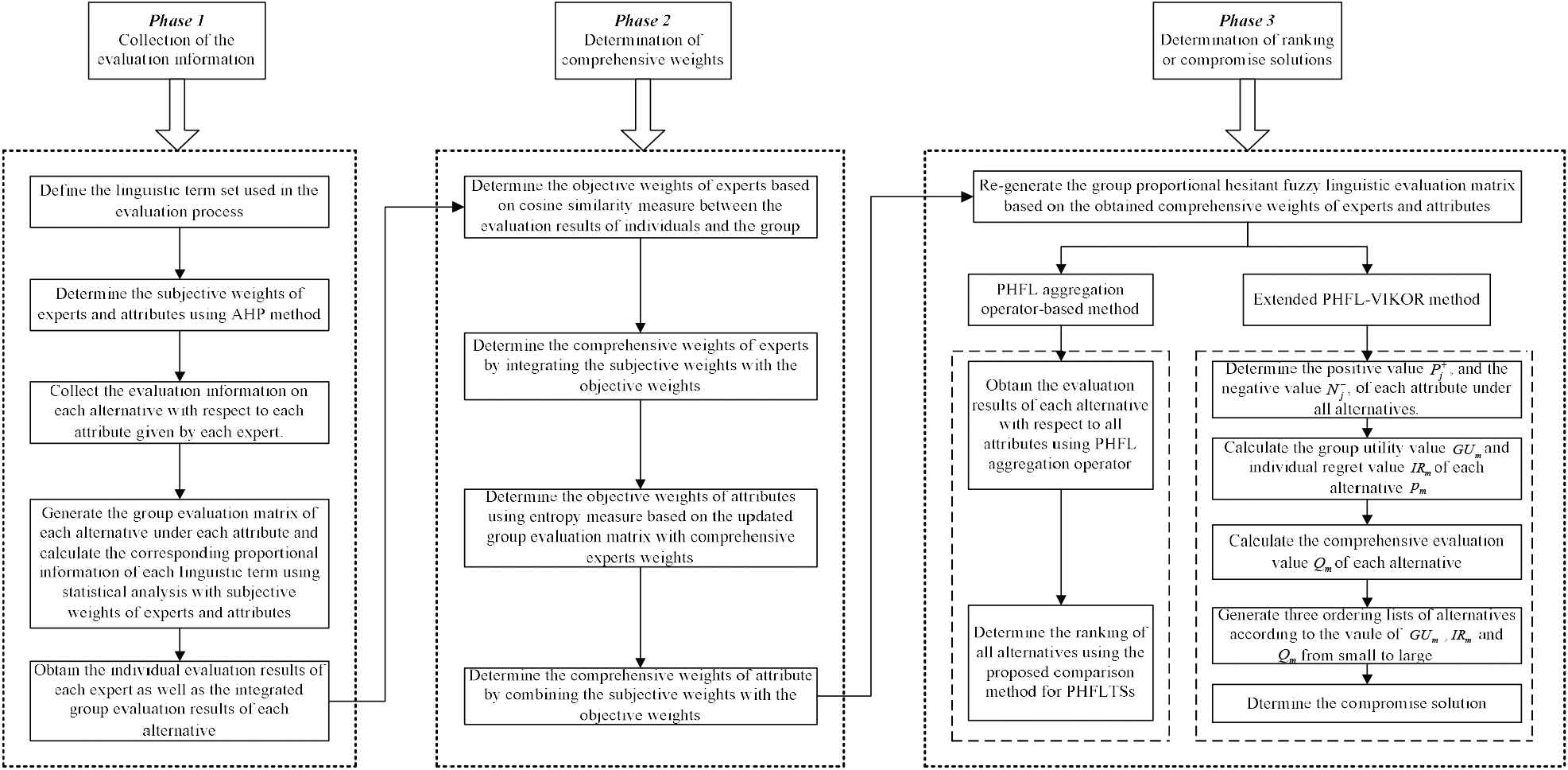
The three-phased schematic of the proposed multi-attribute group decision-making (MAGDM) method.
6. NUMERICAL EXAMPLE
A practical decision-making problem adapted from Parreiras et al. [47] is used to demonstrate the applicability and effectiveness of the two proposed MAGDM methods. The problem is related to making plans for the development of large-scale projects (strategy initiatives) for the next five years by the company's board of directors composing of five members (i.e.,
6.1. PHFLWA Aggregation Operator-Based MAGDM Method
Step 1. Define the LTS and the specific meaning of each linguistic term used in the decision-making process.
Assuming that the sub-script symmetric LTS used in the problem is
Step 2. Determine the subjective weights of experts and attributes using the AHP method.
The top DM of the company provides his evaluation of the importance of experts and attributes using a 1–5 ratio scale. The subjective importance judgment matrices of experts and attributes are shown in Table C.1 (see Appendix C), respectively. After computation, the subjective weights vector of experts is
Step 3. Collect the evaluation information on each alternative with respect to each attribute given by each expert.
The initial individual HFL evaluation matrices given by the five experts are displayed in Tables C.2–C.6 (see Appendix C).
Step 4. Generate the group evaluation matrix of each alternative under each attribute, and calculate the proportional information of each linguistic term in the group evaluation matrix using statistical analysis based on the subjective weights of experts and attributes.
The group PHFL evaluation matrix can be obtained by integrating these five single matrices with proportional information of each occurred linguistic term using statistical analysis method. The result refers to Table C.7 (see Appendix C).
Step 5. Obtain the individual evaluation results as well as the integrated group evaluation results of each alternative under all attributes provided by each expert.
The evaluation results are shown in Table C.8 (see Appendix C).
Step 6.1. Determine the objective weights of experts based on the cosine similarity measure between each expert and group according to Eqs. (16) and (17). Then, we have the objective weights vector of experts
Step 6.2. Determine the comprehensive weights of experts by integrating the subjective weights with the objective weights according to Eq. (18). Here we let
Step 6.3. Determine the objective weights of attributes based on entropy measure according to Eqs. (20) and (21). Then, we have the objective weights vector of attributes
Step 6.4. Determine the comprehensive weights of attributes by combining the subjective weights with the objective weights according to Eq. (22). Here we let
Step 7. Re-generate the group PHFL evaluation matrix based on the obtained comprehensive weights of experts and attributes using the PHFLWA operator proposed in Section 3.3.
The group PHFL evaluation matrix based on the obtained comprehensive weights of experts and attributes is shown in Table 1.
HFL, proportional hesitant fuzzy linguistic.
Group PHFL evaluation matrix based on comprehensive weights of experts and attributes.
Step 8. Determine the ranking of all alternatives.
Step 8.1. Based on the addition operation law of PHFLTSs that proposed in Section 3.2, the overall score of each alternative under all attributes could be calculated.
The evaluation results of each alternative are shown as follows:
Then, using the comparison method for PHFLTSs proposed in Section 3.1, we have
6.2. Extended PHFL-VIKOR Method
Step 1 ~ Step 7. The process and results of Step 1 to Step 7 are the same as those in Section 6.1.
Step 8. Determine the positive value,
Based on Table 1 and Eqs. (23) and (24), we have the positive value of each attribute under all alternatives as follows:
Accordingly, the negative value of each attribute under all alternatives is
Step 9 ~ Step 11. Calculate the group utility value
According to Eqs. (25)–(27), the results of the above aspects are shown in Table 2.
| Ranking | Ranking | Ranking | ||||||||
|---|---|---|---|---|---|---|---|---|---|---|
| 0.0145 | 0 | 0 | 0.021 | 0.759 | 2 | 0.572 | 3 | 0.893 | 3 | |
| 0.0135 | 0.01 | 0.0151 | 0.0125 | 0.880 | 3 | 0.342 | 2 | 0.692 | 2 | |
| 0 | 0.0218 | 0.0065 | 0 | 0.315 | 1 | 0.198 | 1 | 0 | 1 | |
| 0.0145 | 0.0218 | 0.0151 | 0.0125 | - | - | - | - | - | - |
Calculation process and results of
Step 12. Determine the compromise solution.
From Table 2, it is obvious that
From the results obtained by the above two methods, we could clearly see that both of them chose the
6.3. Discussion
In order to demonstrate the influence of the weights of experts and attributes on the decision results, three different ways of combining the weights of experts and attributes are used to derive the results of the same example above. The first way, denoted as w-1, is to use the objective weights of experts and the objective weights of attributes for deriving the decision results in an MAGDM problem. The second way, denoted as w-2, is to use equal weights of experts and subjective weights of attributes. The third way, denoted as w-3, is to use the comprehensive weights of experts and attributes. The results of using the two proposed methods under different ways of combining the weights of experts and attributes are shown in Table 3 and Figure 2.
| Method | Weights Combination Way | Decision-Making Results |
Optimal Alternative | ||
|---|---|---|---|---|---|
| x2 | |||||
| PHFLWA aggregation | w-1 | ||||
| operator | w-2 | ||||
| w-3 | |||||
| w-1 | |||||
| Extended PHFL-VIKOR | w-2 | ||||
| w-3 | |||||
Computational results of PHFLWA aggregation operation operator and Extended PHFL-VIKOR under different ways of combining the weights and attributes.

Comparison on different combination ways of expert weights and attribute weights using proportional hesitant fuzzy linguistic weighted averaging (PHFLWA) aggregation operator-based method.
The results in Table 3 and Figure 2 show that whenever using the PHFLWA aggregation operator-based method or the extended PHFL-VIKOR method,
6.4. Comparison
To demonstrate the necessity of deriving the comprehensive weights of experts and attributes as well as incorporating the proportional information in MAGDM problem under hesitant fuzzy linguistic environment, the example researched by Wang [8] is adopted. This problem relates to the tenure and promotion evaluation of university faculty. Three attributes, including teaching (
Using the proposed extended PHFL-VIKOR method to deal with the problem, the following steps are conducted.
Step 1. Define the LTS and the specific meaning of each linguistic term used in the decision-making process.
Wang [8] defined the LTS used to evaluate the five faculty candidates as
Step 2. Determine the subjective weights of experts and attributes.
The weights of experts and attributes are given by the authors directly in the original example. Therefore, we regard them as the subjective weights. From the description of the problem, it could be seen that the importance of experts in Group 1 is 1.5 times of that of Group 2. We, thus, can reasonably infer that the subjective weight vectors of experts and attributes are
Step 3. Collect the evaluation information on each alternative with respect to each attribute given by each expert.
The evaluation information represented by EHFLTSs given by each expert is depicted in Table C.9 (see Appendix C).
Step 4. Generate the group evaluation matrix of each alternative under each attribute, and, calculate the proportional information of each linguistic term in the group evaluation matrix using statistical analysis based on the subjective weights of experts and attributes.
Based on the subjective weights of experts and attributes, the group PHFL evaluation matrix, shown in Table 4, could be obtained by integrating the five single matrices given by experts using statistical analysis method.
PHFL Evaluation matrix of the group with subjective weights of experts and attributes.
Step 5. Obtain the individual evaluation results as well as the integrated group evaluation results of each alternative under all attributes.
The evaluation results are shown in Table C.10 (see Appendix C).
Step 6.1. Determine the objective weights of experts based on the cosine similarity measure.
According to Table C.10 and Eqs. (16) and (17), we have the objective weight vector of experts
Step 6.2. Determine the comprehensive weights of experts.
Based on the Eq. (18) and let
Step 6.3. Determine the objective weights of attributes based on entropy measure for PHFLTSs.
According to Eqs. (20) and (21), we have the objective weight vector of attributes
Step 6.4. Determine the comprehensive weights of attributes.
Based on the Eq. (22) and let
Step 7. Re-generate the group PHFL evaluation matrix based on the obtained comprehensive weights of experts and attributes using the PHFLWA operator proposed in Section 3.3.
The re-generated group evaluation matrix represented by PHFLTSs, and, based on the obtained comprehensive weights of experts and attributes is shown in Table C.11 (see Appendix C).
Step 8. Determine the positive value,
According to Table C.11 and Eqs. (23) and (24), the positive value and the negative value of each attribute under all alternatives are as follows:
Step 9 ~ Step 11. Calculate the group utility value
According to Eqs. (25)–(27), the group utility value
Step 12. Determine the compromise solution.
It is obvious that
The best alternative obtained by Wang [8] is
6.5. Sensitivity Analysis
When deriving the comprehensive evaluation value of alternatives with the VIKOR method, there is a coefficient
The change process of each alternative's comprehensive evaluation values is shown in Figure 3.

The change process of alternative's comprehensive value with different value of
From Figure 3, we could clearly see that the comprehensive evaluation value of alternative
7. CONCLUSIONS
In order to obtain reliable and accurate results in MAGDM problems, there are two aspects that worth special attention. The first aspect is to retain more initial information from DMs and to reduce the information loss and distortion during the calculation process. The second aspect is how to reasonably determine the weights of experts and attributes as they would have a great influence on the final decision results. To address the first aspect, the concept of PHFLTSs that would simultaneously consider the linguistic terms and proportional information is introduced by this study. When dealing with the second aspect of determining reasonable weights of experts and attributes, a novel comprehensive weighting model, considering not only the subjective weights but also the objective weights, under PHFL environment has been proposed based on the cosine similarity measure and the entropy measure for PHFLTS. Based on the comprehensive consideration of the above two critical aspects, two MAGDM methods, that is, PHFLWA aggregation operator-based method and extended PHFL-VIKOR method are proposed by this study.
The main contributions of this study are as follows:
This study proposed the mathematical normalization method for PHFLTSs. For those PHFLTSs with proportions not equal to one, it is necessary to first normalize the proportions to one uniformly. After that, the cardinality of PHFLTSs should be normalized to be equal for the convenience of computation.
This study proposed some novel basic operations for PHFLTSs. For simplifying the computation process and improving the availability, some operational laws based on the normalized PHFLTSs are proposed, including comparison, arithmetic operations, cosine similarity and distance measures, entropy measure, besides PHFLWA, and PHFLOWA aggregation operators for PHFLTSs.
A comprehensive weighting method under the PHFL environment is proposed. Based on the cosine similarity measure for PHFLTSs, the objective weights of experts are derived. Then, the comprehensive weights of experts are obtained by combining the subjective weights and the objective weights. Entropy measure for PHFLTS is also proposed to determine the objective weights of attributes. The comprehensive weights of attributes are obtained by integrating the subjective weights of attributes with the objective weights of attributes using a simple linear weighting method.
To facilitate decision-making, two MAGDM methods, PHFL aggregation operator-based method and extended PHFL-VIKOR method, with PHFL information are developed. The provision of an illustrative example about large-scale projects development and a comparison example about university faculty evaluation helps showing the feasibility, effectiveness, and advantages of the proposed methods.
For future research, the defined basic operational laws for PHFLTSs could be used to develop novel aggregation functions, such as those in Ref. [49–51], and other MAGDM methods with PHFL information. Development of large-scale group decision-making methods with preference relations, similar to Ref. [52], under PHFL environment is also an interesting topic.
CONFLICT OF INTEREST
The authors declare that they have no known competing financial interests or personal relationships that could have appeared to influence the work reported in this paper.
Funding Statement
This study was supported by the Cultivation Program for the Excellent Doctoral Dissertation of Southwest Jiaotong University (D-YB201905), the RGC TBRS project (Grant No. T32-101/15-R), the Ger/HKJRS project (Grant no. G-CityU103/17), the City University of Hong Kong SRG (Grant no. 7004969), and the National Natural Science Foundation of China (Grant nos. 71971182, 71872153, 71371156).
AUTHORS' CONTRIBUTIONS
Qiang Yang is a team member of the research project. In the research, he participated in determining the research idea, constructing the model, calculating and analyzing the results, and writing the paper; Yan-Lai Li is a team member of the research project. In the study, he helped to write the paper and to provide a part of funding supports for the research.
Kwai-Sang Chin is a team member of the research project. In the study, he participated in suggesting the research idea, polishing the English of the paper and providing a part of funding supports for the research.
ACKNOWLEDGMENT
This study was supported by the Cultivation Program for the Excellent Doctoral Dissertation of Southwest Jiaotong University (D-YB201905), the RGC TBRS project (Grant No. T32-101/15-R), the Ger/HKJRS project (Grant no. G-CityU103/17), the City University of Hong Kong SRG (Grant no. 7004969), and the National Natural Science Foundation of China (Grant nos. 71971182, 71872153, 71371156).
APPENDIX A
Proof of Theorem 2.
Proof.
The proof for Theorems (1) and (2) are omitted here as they are obviously satisfied.
APPENDIX B
Proof of the proposed cosine similarity exhibits the axioms.
Proof.
The proof of axiom (1) and (3) are omitted here as they are obviously satisfied. We only need to demonstrate the axiom (2), that is
Based on the Definition 16, we have
APPENDIX C
| Experts | Attributes | |||||||||
|---|---|---|---|---|---|---|---|---|---|---|
| 1 | 1/2 | 1/2 | 1/2 | 1 | 1 | 1/2 | 1/4 | 1 | ||
| 2 | 1 | 1/2 | 1/2 | 2 | 2 | 1 | 1 | 2 | ||
| 2 | 2 | 1 | 2 | 3 | 4 | 1 | 1 | 3 | ||
| 2 | 2 | 1/2 | 1 | 1 | 1 | 1/2 | 1/3 | 1 | ||
| 1 | 1/2 | 1/3 | 1 | 1 |
The evaluation matrix for determining the subjective importance of experts and attributes.
The hesitant fuzzy linguistic evaluation matrix that given by
The hesitant fuzzy linguistic evaluation matrix that given by
The hesitant fuzzy linguistic evaluation matrix that given by
The hesitant fuzzy linguistic evaluation matrix that given by
The hesitant fuzzy linguistic evaluation matrix that given by
Group PHFL evaluation matrix based on subjective weights of experts and attributes.
Evaluation results of each alternative.
Evaluation matrix given by
Evaluation results of each alternative represented by PHFLTSs.
Re-generated group PHFL evaluation matrix.
REFERENCES
Cite this article
TY  - JOUR
AU  - Qiang Yang
AU  - Yan-Lai Li
AU  - Kwai-Sang Chin
PY  - 2019
DA  - 2019/09/18
TI  - Constructing Novel Operational Laws and Information Measures for Proportional Hesitant Fuzzy Linguistic Term Sets with Extension to PHFL-VIKOR for Group Decision Making
JO  - International Journal of Computational Intelligence Systems
SP  - 998
EP  - 1018
VL  - 12
IS  - 2
SN  - 1875-6883
UR  - https://doi.org/10.2991/ijcis.d.190902.001
DO  - 10.2991/ijcis.d.190902.001
ID  - Yang2019
ER  -