
Heterogeneous Interrelationships among Attributes in Multi-Attribute Decision-Making: An Empirical Analysis
- DOI
- 10.2991/ijcis.d.190827.001How to use a DOI?
- Keywords
- Heterogeneous interrelationships; Generalized extended Bonferroni mean; Simple additive weighting; Preference modeling; Multi-attribute decision function
- Abstract
Tremendous effort has been exerted over the past few decades to construct multi-attribute decision functions with the capacity to model heterogeneous interrelationships among attributes. In this paper, we report an empirical study aiming to test whether or not considering interrelationships among attributes can benefit the representation of real preferences in multi-attribute ranking tasks. The generalized extended Bonferroni mean (GEBM) has recently been advocated as a promising and efficient tool for modeling heterogeneous interrelationships among attributes. We compare the GEBM with one of its most widely adopted competitors, simple additive weighting (SAW), in terms of their fitting quality when applied to preference elicitation. The attribute performances are manifested uniformly with the use of three widely-adopted utility measurements. Subsequently afterwards, the maximum split approach to establish the constraint objective function in regression for both the GEBM and the SAW to test whether or not all constraints resulting from the subject’s ranking can be fulfilled. On this bases, the number of fully or partly fitted subjects, consistency for subjects according to the better fitting model, and reliability of attribute weights learned by either the GEBM or the SAW are empirically examined in a bid to demonstrate the quantitative construction of fitting quality measurement. With the established fitting quality measurement, the necessity of taking heterogeneous interrelationships among attributes into account when constructing multi-attribute decision functions to represent real preferences can be analyzed. The main conclusion from the empirical study suggests that the relative performance of the two aggregation paradigms examined here depends on which fitting quality measurements are adopted. Researchers enthusiastic to discover the heterogeneous interrelationships among attributes when constructing multi-attribute decision functions might find the present results relevant when modeling actual preferences, and consequently this work should serve as a useful reference for enterprises and service providers seeking to strategically drive customer purchasing decisions.
- Copyright
- © 2019 The Authors. Published by Atlantis Press SARL.
- Open Access
- This is an open access article distributed under the CC BY-NC 4.0 license (http://creativecommons.org/licenses/by-nc/4.0/).
1. INTRODUCTION
Typical multi-attribute decision-making (MADM) structures often involve the following three components: (1) evaluation of various alternatives against certain attributes, (2) determination of the attributes weights reflecting the preference of a decision maker, and (3) aggregation of the attributes evaluations taking account of the attributes weights [1]. A considerable number of MADM methodologies and theories have been developed and applied in a wide range of fields, such as bid evaluation, enterprise strategy planning, quality assessment, and product recommendation [2–7]. However, in many decision-making scenarios, decision makers do not always follow the above procedures in a stepwise manner, since they usually have some rough idea in the first place of the appropriate outputs for some prototype inputs [8,9]. The preference aggregation outputs are usually in the form of numerical data or preferences (e.g., expressed as linear orderings). For example, a decision maker can offer a ranking of cars
Identification of aggregation functions for preference modeling and elicitation of attributes weighting vectors have been hot research topics for the past few decades [10–15]. Recent efforts in this area have been devoted to the incorporation of the human cognitive process by fitting different types of aggregation functions to empirical data collected from real-life scenarios. Reimann et al. [16] fitted the ordered weighted averaging (OWA) and simple additive weighting (SAW) models to empirical data. In general, the OWA model gives a slightly poorer fit to empirical data. The use of empirical studies has brought a novel perspective to the preference modeling field, allowing the examination of a huge amount of research data on the aggregation of attributes evaluations. Motivated by [16], this paper initiates an additional effort to test another question: “Can considering heterogeneous interrelationships among attributes in multi-attribute decision functions provide a better representation of real preferences?” In particular, heterogeneous interrelationships among attributes in the context of MADM reveal a situation in which both dependency and independency implicitly coexist in the attribute structure and need to be simultaneously taken into consideration, which are demonstrated in recent research efforts to be a significant factor affecting the decision-making process [17,18]. In real-life MADM problems, there usually exist complex interrelationships among the attributes under consideration, which are reflected in the corresponding input arguments [8,16,19]. For example, consider a car choice problem where four attributes, namely, price (
The solution to this problem requires the use of several prominent aggregation functions to model the interrelationships among attributes in the construction of multi-attribute decision functions. The Choquet integral (CI) proposed in [20] and the power average (PA) operator introduced in [21] are useful tools to model the interdependence or correlation among input arguments. However, both focus on capturing interrelationships among input arguments depending on the fuzzy measure (FM) determination and the support function construction. The appropriate choice of FM and support function is still a matter of debate, and, in particular, the PA operator can only be used for modeling homogeneous interrelationships [19]. The generalized extended Bonferroni mean (GEBM), which originates from the Bonferroni mean (BM), has been advocated in the recent literature as a promising and efficient tool for modeling heterogeneous interrelationships among attributes. To simplify our empirical study, the GEBM and its competing SAW model are selected when modeling such interrelationships in multi-attribute decision functions to facilitate an explicit discussion of their different aggregation paradigms.
The BM has been one of the most powerful aggregation functions in the field of MADM since its introduction by Bonferroni in [22] in 1950. Owing to the inherent structure of the BM, it can model homogeneous correlations among attributes by connecting each argument with other arguments [8]. On the basis of this property, Dutta et al. [23] extended the BM to accommodate even more complex correlations among attributes where some arguments are related to only a nonempty subset of the remaining arguments, while others have no relation to the remaining arguments; this is termed the extended BM (EBM). As a structural generalization of the EBM, the GEBM proposed by Chen et al. [24] allows heterogeneous interrelationships among aggregation inputs to be effectively captured in a more flexible way in situations where both dependent and independent attributes need to be simultaneously taken into consideration. Compared with other aggregation functions capable of modeling interrelationships among attributes, one of the main advantages of the GEBM is that it can be identified as a composite function consisting of averaging and conjunctive operators. The aggregation mechanism is reflected by the composite function, which is convenient for decomposition and substitution with restricted forms of aggregation functions. The specific requirements for various applications can be satisfied by defining appropriate composite aggregation functions, which makes the GEBM one of the most useful aggregation functions in the context of decision-making. The GEBM has attracted a great deal of attention with regard to its theoretical development since its introduction in [23], no work has been done on its fitting to empirical data that represent the real preferences of decision makers [1,25]. In addition, it has yet to be applied to test whether considering interrelationships among attributes can provide a better representation of real preferences.
To fill this research gap, this paper conducts a large-scale empirical study to fit the GEBM and the SAW respectively to empirical data and to test whether considering interrelationship among attributes can indeed provide a better representation of real preferences. There are three main components of this procedure: aggregation functions, attributes evaluations and rankings provided by survey respondents, and constraint functions in regression. In our experiment, for comparison with the GEBM, we use SAW as a benchmark preference-approximation model in which interrelationships among attributes are not considered. More specifically, we provide the performance parameters of products as model inputs and ask the subjects for the rankings of alternative products as outputs. The rankings of alternatives include richer information compared with that obtained from the choice and sorting tasks, and are easier to obtain in real-word scenarios in comparison with accurate aggregated scores. To derive feasible weighting parameters for each model, a maximum split approach is used as the constraint function in regression.
The remainder of the paper is structured as follows. A review of the literature on identification of aggregation functions and elicitation of weighting vector is presented in Section 2. Section 3 provides several definitions of the BM, GBM, and GEBM, and the other two main components used in the development of our proposed approach. We describe our experimental design and data collection in Section 4. In Section 5, a comparison of fitting quality for the GEBM and SAW models is given. Section 6 concludes the paper.
2. LITERATURE REVIEW
The developments of this empirical study consist mainly of (a) aggregation functions for attribute interrelationships elicitation, (b) fitting aggregation functions to empirical data, and (c) detailed analysis of empirical results. As such, the literature review is subdivided as follows.
Aggregation functions for attribute interrelationship elicitation.
In term of the interactions among attributes in MADM, the attribute interrelationships can be categorized into two groups: the homogeneity and heterogeneity [8,26,27]. Homogeneous interrelationship means that given a set of attributes
Except for the BM and its generalizations, there exist a considerable amount of aggregation functions capable of modeling different type of attribute interrelationships. Among the existing aggregation functions, CI is commonly considered as one of the most powerful tools for aggregating interacting attributes as an adequate substitute to weighted arithmetic mean or OWA operator [28,29]. CI introduces the renowned concept of FM to allow defining weights of attributes not only on the single-attribute level, but also on each subset of attributes in a nonadditive fashion. FM on each combination of attributes is measured by importance index and interaction index of attributes, thus making it possible to model the interactions among attributes [30]. To take into account the interrelationship between the input arguments in an information fusion, Yager [21] introduced the concept of the PA operator, as mentioned before. In its inherent structure, the PA operator when applied to MADM scenario assumes that the weight of an attribute depends on the interrelationship between this attribute and all the remaining attributes, which is accomplished by calculating the support value from the rest to each attribute, following the simple philosophy that the more similar two attribute inputs are, the more they support each other [26]. Heronian mean (HM) is characterized by the ability to capture the relevance between arguments, which has also been regarded as a useful tool to model attribute interrelationships. Compared with the BM, HM assumes that the self-interaction should be incorporated in the aggregation of attributes, and it distinguishes the interrelationship between attributes
Fitting aggregation functions to empirical data.
There have been a number of papers related to fitting aggregation functions with empirical data. Beliakov [11] studied methods for fitting weighted arithmetic means, OWA functions, and CIs, and showed that the linear programming formulation is valid for such cases. Weighted quasi-arithmetic means and OWA functions were identified and described, together with their corresponding weighting vectors, in [13,14,35,36]. Kumar and Tripathi [37] fitted two new aggregation functions called compensatory summation units (CSUs) and compensatory product units (CPUs). Reimann et al. [16] fitted OWA and SAW models to empirical data to test how well the OWA operator represents real preferences. A comprehensive overview of methods for capacity identification in Choquet-integral-based multi-attribute utility theory was conducted in [38], using the Kappalab R package. Beliakov [39] proposed an approach for fitting triangular norms and conorms to empirical data in which membership functions and aggregation operators were constructed from the data, and they applied it to fuzzy systems. Other aggregation functions fitted in fuzzy control were studied in [40–42]. The fitting process is often related to information from inputs and outputs. Various types of inputs and outputs have been introduced to fit aggregation functions. Typically, inputs and outputs are real numbers, often from the range [0, 1], although other choices are possible, such as discrete sets, intervals, and linguistic labels. In [1,16,43], real numbers were used as inputs and ranking preferences as outputs, and the fitting process was conducted after the inputs had been normalized. Beliakov [11] employed real numbers and the desired overall aggregation scores of each alternative as inputs and outputs, respectively. Beliakov [11] and Shepetukha and Olson [44] introduced a fitting method with interval-valued inputs. The constraint function in regression is also an important part of the fitting procedure. Here, we concentrate on linear programming problems. Grabisch et al. [38] provided a comprehensive overview of constraint functions used for capacity identification in the CI. Beliakov [11] used the “least absolute deviation” attributes proposed by Bloomfield and Steiger [45] as a constraint objective function that minimizes the deviation between aggregated score and desired score. A maximum entropy and minimum variance principle for capacities was introduced by [46–48]. Reimann et al. [16] maximized the deviation of aggregation scores between two different alternatives in different orders, while Ahn [10] used the sum of deviations as an objective function. Geng et al. [49] and Khot et al. [50] argued that approximation algorithms have achieved success in empirical applications. Jiang et al. [48] proposed a weight learning method for medical knowledge networks based on a max-margin framework.
By fitting aggregation functions to empirical data, we can often obtain the weighting vector of attributes, which is a core product of the fitting process. In fact, instead of using a fitting process, many studies have obtained the attribute weights by comparisons of attribute importance [51]. In the approach of Shepetukha and Olson [44], attribute weights were learned using the ranking of attribute importance and the relative weights between adjacent attributes. Solymosi and Dombi [52] compared attribute importance by considering threshold values and introduced the centroid of the feasible set of formulated linear inequalities as a weighting vector for attributes. Mikhailov [53] decomposed the fuzzy comparison judgments of attributes into a series of interval judgments by using
| Aggregation Functions | Inputs | Outputs | Objective Functions | Ref. |
|---|---|---|---|---|
| OWA, SAW | Real numbers | Ranking | Maximum split | [16] |
| Choquet integrals, triangular norms and conorms | Interval values | Interval values | Least absolute deviation | [11] |
| AM/GM/QM/OWA/GBM/Choquet integrals | Real numbers | Desired overall score/ranking | Least absolute deviation/maximum split | [12] |
| OWA | Real numbers | Ranking | Maximum likelihood | [1] |
| Choquet integrals | Real numbers | Desired overall score/ranking | Least squares/maximum split/minimum variance/minimum distance | [38] |
OWA, ordered weighted averaging; SAW, simple additive weighting; GBM, generalized Bonferroni mean.
Research on fitting aggregation functions to empirical data.
Analyses of empirical data.
Different proposals have adopted distinct approaches to obtain useful insights from analyses of empirical data. Reimann et al. [16] employed measurements of the consistency between ranking and valuation tasks and between two ranking tasks, the Cognitive Style Index, the fitting ability of rankings of subsets, and the distributions of weights. To test fitting ability, Beliakov et al. [12] applied the percentage of comparisons accurately predicted using various aggregation functions, as well as the results of fitting aggregation functions to raw abundance data. Beliakov and James [55] introduced 10-fold cross-validation accuracy to test the adaptability of aggregation functions. Grabisch et al. [38] analyzed the distributions of weights of different constraint objective functions in regression for empirical results.
3. PRELIMINARIES
In this section, we set out to introduce the necessary background on the SAW and GEBM. After giving some important definitions and properties, we present our constraint objective function and linear constraints in regression for SAW and GEBM. More detailed overviews of aggregation functions can be found in [56,57], and, without further specifications, this paper follows roughly the notation used in [8,27].
Definition 1.
[56] A function
Aggregation functions are classified depending on their behavior with respect to inputs [58]. An aggregation function
Definition 2.
[56] For a given strictly monotone and continuous function
In particular, if the generating function is
The SAW method, also known as the weighted sum method, is the most widely used MADM method [59]. The basic principle of SAW is to obtain a weighted sum of the performance ratings of each alternative under all attributes [60]. The SAW method consists of two basic steps [59,60]: (1) scale the values of all attributes to make them comparable; (2) aggregate the values of all the attributes for each alternative with weighted average mean operator.
As an effective aggregation function, the BM has been successfully applied in such fields as image processing [61,62], environmental modeling [63], water quality analysis [24], and social network analysis [64]. The BM has such a wide range of applications because of its decomposable structure and distinguishable components. Its original functional form is composed of two averaging operators and a conjunctive operator that can be interpreted as involving a product of each argument with the average of the other arguments [65].
Definition 3.
[22] Let
The BM is an averaging aggregation operator. It can be interpreted as computing the average satisfaction of each input
As an extension of this basic concept, Yager [65] replaced the simple average operator by other types of mean aggregation function such as the OWA function and the discrete CI and introduced arguments with varying importance weights. Beliakov et al. [66] then studied various weighted quasi-arithmetic means and t-norm functions to replace the averaging operators and conjunctive function, respectively, and investigated the properties of this generalized BM (GBM).
Definition 4.
[66] Let
Both
Beliakov et al. [66] found that the GBM has sufficient modeling capabilities for the concepts of partial conjunction, partial disjunction,
The GBM refers to a connection of each argument
Definition 5.
[23] For any
As indicated by this formula, the EBM operator is divided into two components: the dependent part (the former) and the independent part (the latter). If
Definition 6.
[8] Let
In addition to aggregation operators, utility measurement is also an important part of the empirical-data-fitting process. In this paper, we use linear, concave and convex utility functions for utility measurement, as suggested in Reimann et al. [16]: linear utility function:
We apply the maximum split approach to establish the constraint objective function in regression, which can be interpreted as
From the general form of the constructed constraint objective function, we can see that only a positive value of the deviation variable
For the GEBM, we use a weighting vector
4. EXPERIMENTAL DESIGN AND DATA COLLECTION
To compare the fitting quality of GEBM and SAW towards empirical data, we took smart phones as the experimental materials because they are widely used and their configuration parameters are easily understood. Students were taken as subjects because the majority of students possess at least one smart phone. In this experiment, we provided various configuration parameters of several smart phones and asked the subjects to rank these phones according to their preferences. To avoid any influence of brand effect on our empirical results, we did not include any brand information on the experimental materials in the questionnaire, and no photographs or models were shown to the subjects. We employed the following attributes and configuration parameters.
Battery capacity (
Thickness (
Screen size (
Cruising power (
Camera (
ROM (
A heterogeneous interrelationship can be established on the basis of these six attributes. In general, cruising power is related to battery capacity, screen size, and phone thickness, and a thinner phone often implies a smaller battery capacity. The interrelationships among the attributes are shown in Figs. 1–5. The configuration parameters of the smart phones in our experiment are given in Table 2. Utility measurements are given in Tables 3–5.
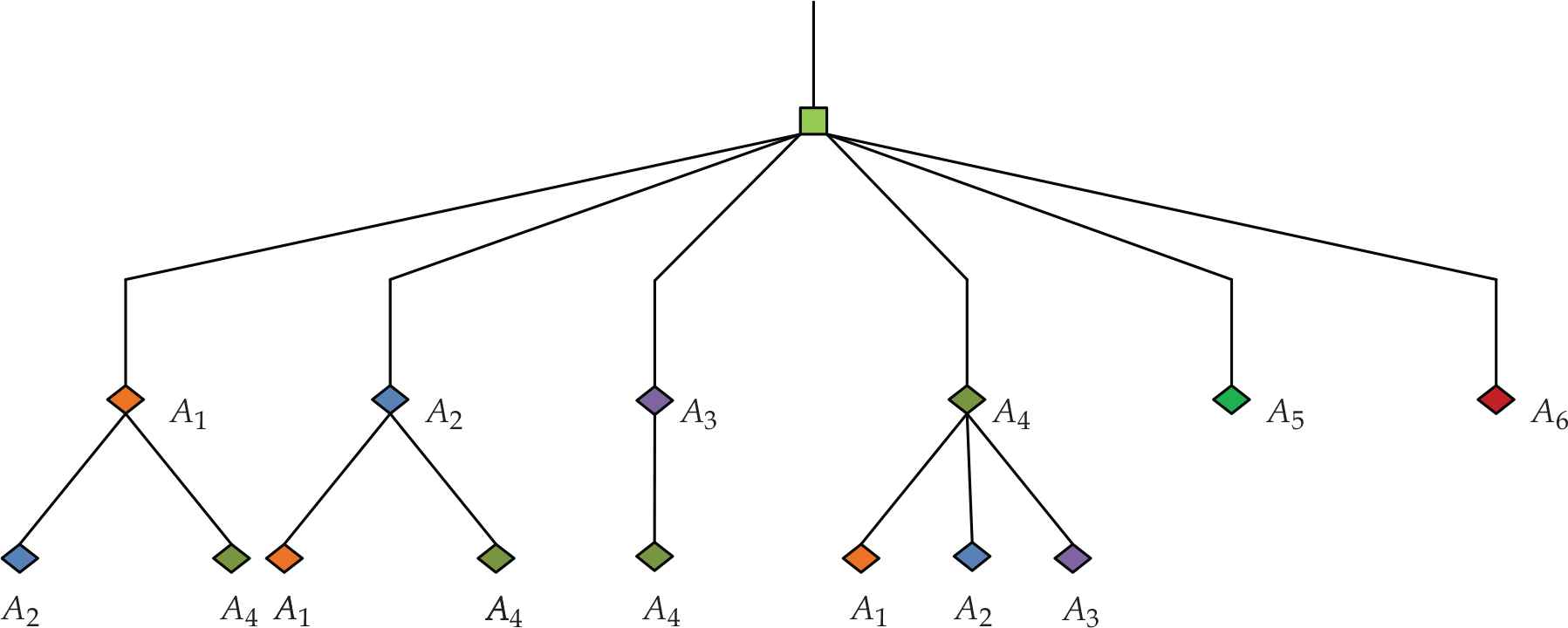
Interrelationships among selected attributes of smart phones.
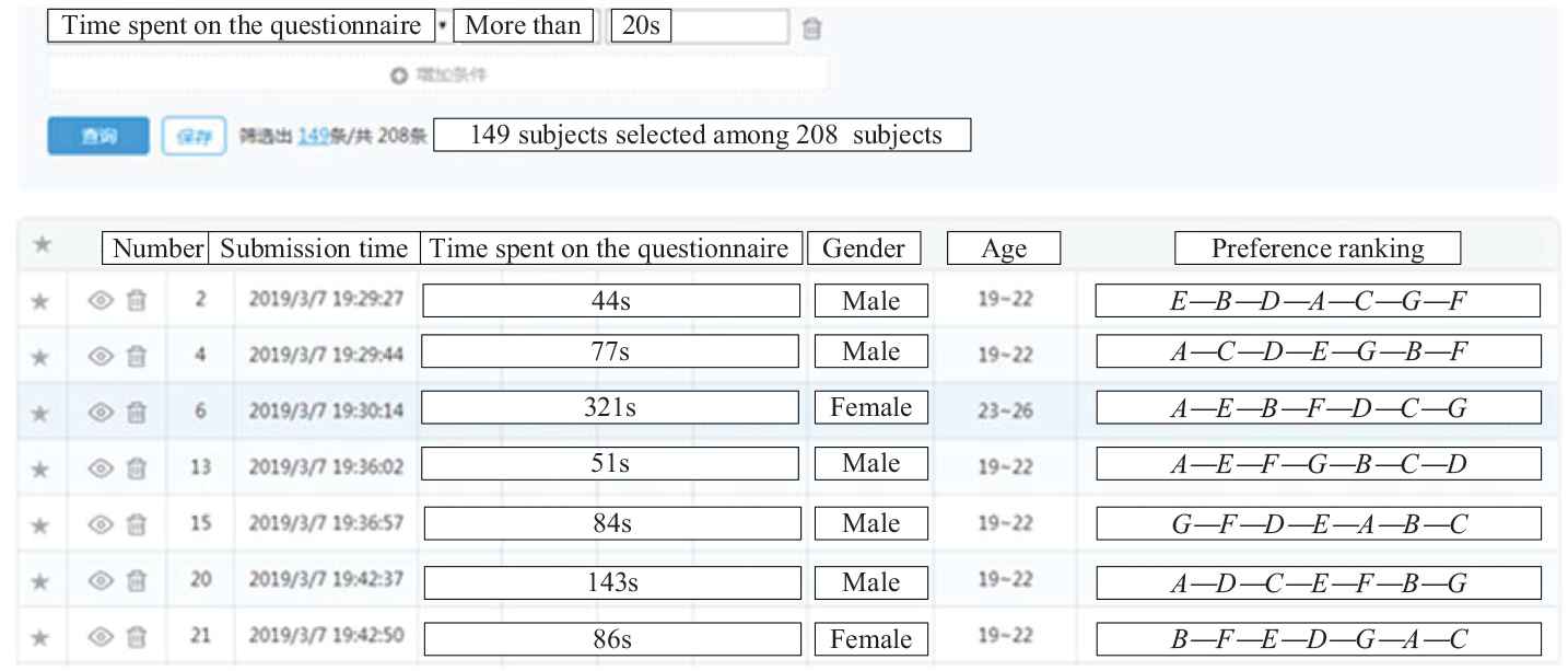
Available questionnaires of survey 1.
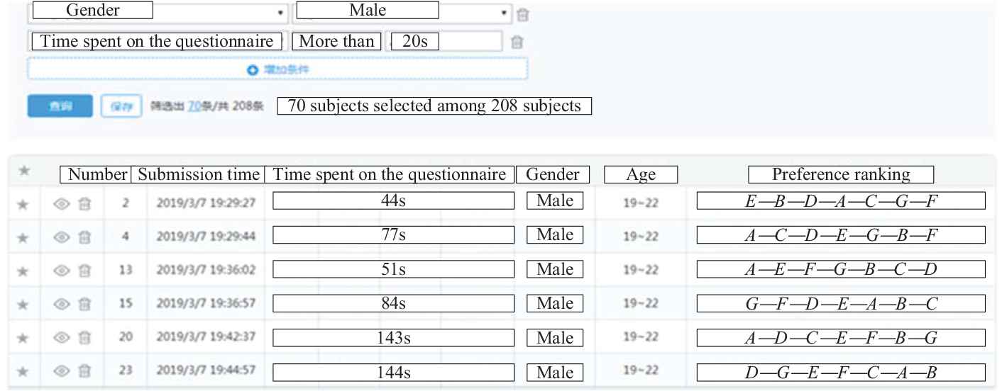
Available male subjects of survey 1.
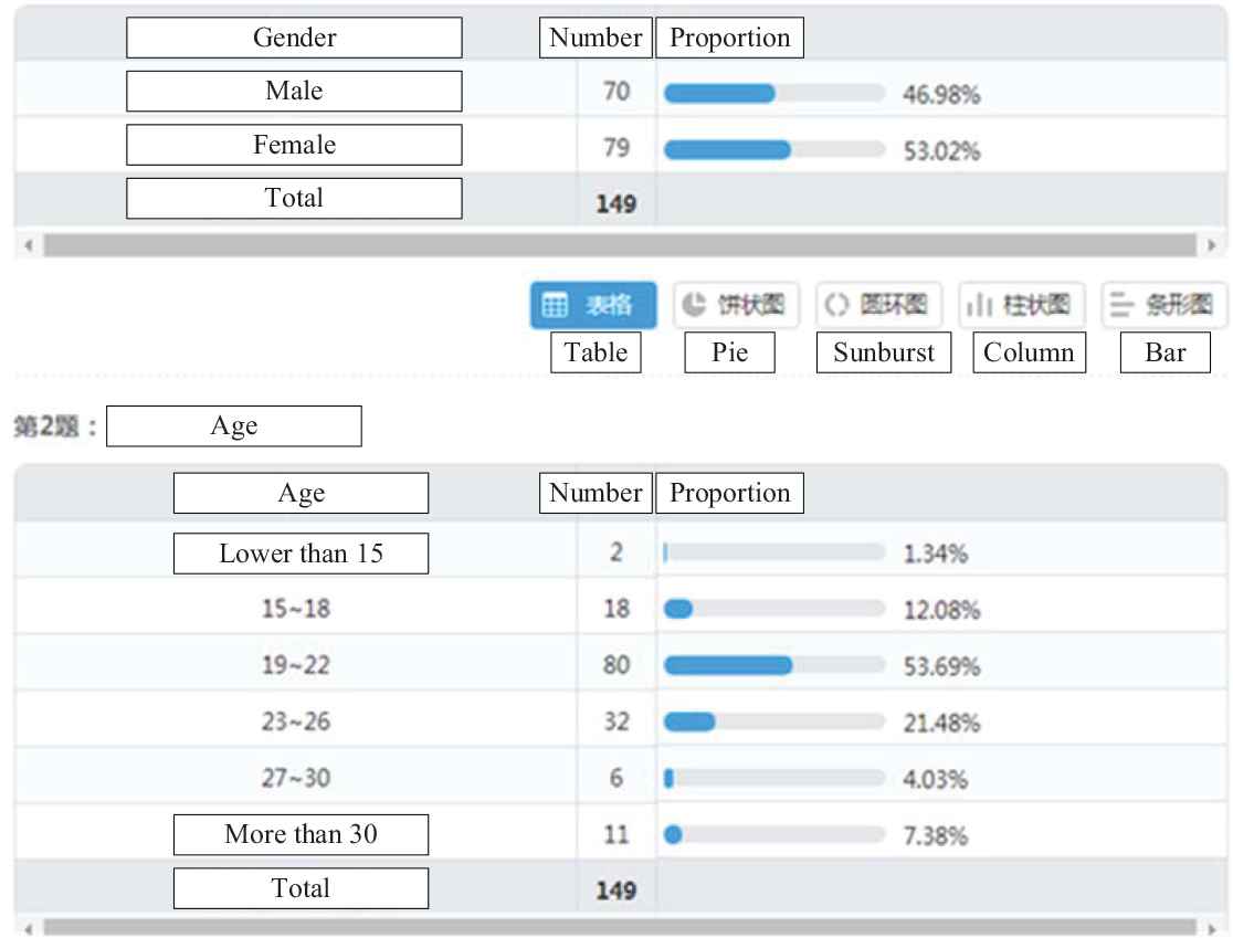
Genders and ages of available subjects of survey 1.
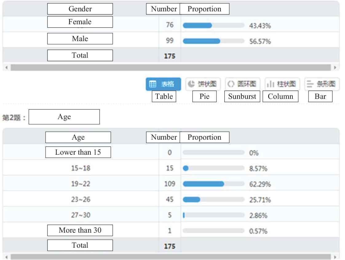
Genders and ages of available subjects of survey 2.
| Smart Phone | Battery Capacity (mAh) | Thickness (mm) | Screen Size (inches) | Cruising Power (hours) | Camera (megapixels) | ROM (GB) |
|---|---|---|---|---|---|---|
| A | 4000 | 7.80 | 6.10 | 7.56 | 20 | 64 |
| B | 3300 | 8.60 | 6.30 | 6.15 | 12 | 128 |
| C | 3500 | 8.50 | 6.20 | 7.18 | 12 | 64 |
| D | 3060 | 11.1 | 5.70 | 7.00 | 19 | 128 |
| E | 3300 | 7.25 | 6.00 | 7.00 | 20 | 128 |
| F | 3520 | 7.62 | 6.00 | 6.00 | 12 | 256 |
| G | 2716 | 7.70 | 5.80 | 6.80 | 12 | 256 |
| 4000 | 7.25 | 6.30 | 7.56 | 20 | 256 | |
| 2716 | 11.1 | 5.80 | 6.00 | 12 | 64 |
Configuration parameters of smart phones.
| Smart Phone | Battery Capacity | Thickness | Screen Size | Cruising Power | Camera | ROM |
|---|---|---|---|---|---|---|
| A | 1.000 | 0.857 | 0.667 | 1.000 | 1.000 | 0 |
| B | 0.455 | 0.649 | 1.000 | 0.096 | 0 | 0.333 |
| C | 0.611 | 0.675 | 0.833 | 0.756 | 0 | 0 |
| D | 0.268 | 0 | 0 | 0.641 | 0.875 | 0.333 |
| E | 0.455 | 1.000 | 0.500 | 0.641 | 1.000 | 0.333 |
| F | 0.626 | 0.904 | 0.500 | 0 | 0 | 1 |
| G | 0 | 0.883 | 0.167 | 0.513 | 0 | 1 |
Linear utility measurement.
| Smart Phone | Battery Capacity | Thickness | Screen Size | Cruising Power | Camera | ROM |
|---|---|---|---|---|---|---|
| A | 1.000 | 0.926 | 0.817 | 1.000 | 1.000 | 0 |
| B | 0.675 | 0.806 | 1.000 | 0.310 | 0 | 0.577 |
| C | 0.782 | 0.822 | 0.913 | 0.869 | 0 | 0 |
| D | 0.518 | 0 | 0 | 0.801 | 0.935 | 0.577 |
| E | 0.675 | 1.000 | 0.707 | 0.801 | 1.000 | 0.577 |
| F | 0.791 | 0.951 | 0.707 | 0 | 0 | 1 |
| G | 0 | 0.913 | 0.409 | 0.716 | 0 | 1 |
Concave utility measurement.
| Smart Phone | Battery Capacity | Thickness | Screen Size | Cruising Power | Camera | ROM |
|---|---|---|---|---|---|---|
| A | 1.000 | 0.766 | 0.449 | 1.000 | 1.000 | 0 |
| B | 0.207 | 0.421 | 1.000 | 0.009 | 0 | 0.111 |
| C | 0.373 | 0.456 | 0.694 | 0.572 | 0 | 0 |
| D | 0.072 | 0 | 0 | 0.411 | 0.766 | 0.111 |
| E | 0.207 | 1.000 | 0.250 | 0.411 | 1.000 | 0.111 |
| F | 0.392 | 0.817 | 0.250 | 0 | 0 | 1 |
| G | 0 | 0.780 | 0.028 | 0.263 | 0 | 1 |
Convex utility measurement.
We conducted our experiment using an online questionnaire that asked three questions of each subject: their gender and age and their preference rankings for the seven smart phones. To improve the analysis, we conducted two surveys under the same conditions. The first survey involved 208 subjects, who took an average time of 87.28 s each to complete the questionnaire. After excluding subjects who completed the questionnaire in less than 20 s, we were left with 149 answers from 70 male (46.98%) and 79 female (53.02%) subjects, with an average age of 21.8 years and an average completion time of 105.05 s. In the second survey, 223 subjects were involved and provided 175 available answers. In this survey, 76 participants (43.43%) were male and 99 (56.57%) female, with an average age of 21.5 years and an average completion time of 94.55 s.
5. COMPARISON OF FITTING QUALITY OF AGGREGATION OPERATORS
According to the empirical surveys designed above, the fitting quality of GEBM and SAW can be compared. In this section, the number of fully or partly fitted subjects, consistency for subjects according to the better fitting model, and reliability of attribute weights learned by either the GEBM or the SAW are empirically examined in a bid to demonstrate the quantitative construction of fitting quality measurement.
5.1. Descriptive Statistics
The responses provided by our subjects were quite heterogeneous. As can be seen from Tables 6 and 7, except for smart phones A and G, the distributions of ranks for the other phones are even, with standard deviations below 10.4 in both surveys, which means that the viewpoint of subjects on ranking is highly decentralized. We can also observe that some alternatives (B and D in both surveys) have almost the same chance of being ranked first and last. Thus, the preferences of the subjects cover a wide range of possible rankings and provide a rich sample to which the two models can be fitted.
| Rank | 1 | 2 | 3 | 4 | 5 | 6 | 7 |
|---|---|---|---|---|---|---|---|
| A | 62 | 18 | 12 | 9 | 8 | 21 | 19 |
| B | 12 | 24 | 22 | 21 | 34 | 24 | 12 |
| C | 12 | 16 | 34 | 15 | 24 | 21 | 27 |
| D | 16 | 19 | 22 | 38 | 24 | 14 | 16 |
| E | 17 | 26 | 30 | 34 | 27 | 12 | 3 |
| F | 20 | 29 | 14 | 15 | 19 | 41 | 11 |
| G | 10 | 17 | 15 | 17 | 13 | 16 | 61 |
Distribution of ranks for all alternatives in survey 1.
| Rank | 1 | 2 | 3 | 4 | 5 | 6 | 7 |
|---|---|---|---|---|---|---|---|
| A | 85 | 18 | 14 | 10 | 12 | 18 | 18 |
| B | 14 | 28 | 26 | 24 | 40 | 28 | 15 |
| C | 9 | 27 | 39 | 27 | 18 | 29 | 26 |
| D | 13 | 23 | 24 | 46 | 32 | 18 | 19 |
| E | 16 | 26 | 32 | 34 | 39 | 21 | 7 |
| F | 21 | 33 | 27 | 18 | 21 | 40 | 15 |
| G | 17 | 20 | 13 | 16 | 13 | 21 | 75 |
Distribution of ranks for all alternatives in survey 2.
To test whether considering interrelationships among attributes can provide a better representation of real preferences, we need to compare the fitting quality of the GEBM operator with that of the SAW model. A comparative analysis between the GEBM and SAW models will be conducted with regard to the following aspects.
5.2. Number of Fully Fitted Subjects
As mentioned above, only a positive
| Linear | Concave | Convex | |
|---|---|---|---|
| Survey 1 | |||
| SAW | 0.1342 | 0.1074 | 0.0805 |
| GEBM | 0.0201 | 0.0067 | 0.0268 |
| Survey 2 | |||
| SAW | 0.0971 | 0.0743 | 0.0801 |
| GEBM | 0.0457 | 0.0229 | 0.0571 |
SAW, simple additive weighting; GEBM, generalized extended Bonferroni mean.
Proportion of positive z.
| Linear | Concave | Convex | |
|---|---|---|---|
| Survey 1 | |||
| SAW | −0.0791 | −0.0706 | −0.0905 |
| GEBM | −0.0834 | −0.0836 | −0.1046 |
| Survey 2 | |||
| SAW | −0.0852 | −0.0699 | −0.1042 |
| GEBM | −0.0834 | −0.0786 | −0.1063 |
SAW, simple additive weighting; GEBM, generalized extended Bonferroni mean.
Mean of z in different models.
From these tables, we observe that the GEBM operator has a lower proportion of positive
5.3. Number of Partly Fitted Subjects
As revealed in Section 5.2, the fits of both aggregation functions to the complete rankings are poor. Therefore, we consider both models with all possible subsets of these alternatives (
From Tables 10–12, we can see that the SAW model fits better for all possible subsets of alternatives. In particular, with increasing subset size, the quality of fit of the GEBM operator falls rapidly, as a result of which it gives a far poorer fit for larger subset sizes. For example, for
| Subset Size | 2 | 3 | 4 | 5 | 6 |
|---|---|---|---|---|---|
| Survey 1 | |||||
| SAW | 0.9741 | 0.9223 | 0.7785 | 0.5407 | 0.2982 |
| GEBM | 0.9111 | 0.7166 | 0.4754 | 0.2557 | 0.1074 |
| Survey 2 | |||||
| SAW | 0.9766 | 0.9298 | 0.7856 | 0.5265 | 0.2678 |
| GEBM | 0.9118 | 0.7159 | 0.4740 | 0.1257 | 0.0457 |
SAW, simple additive weighting; GEBM, generalized extended Bonferroni mean.
Proportion of positive z for alternative subsets with linear utility measurement.
| Subset Size | 2 | 3 | 4 | 5 | 6 |
|---|---|---|---|---|---|
| Survey 1 | |||||
| SAW | 0.9741 | 0.9108 | 0.7421 | 0.4775 | 0.2378 |
| GEBM | 0.9112 | 0.7093 | 0.4740 | 0.2432 | 0.0911 |
| Survey 2 | |||||
| SAW | 0.9767 | 0.9207 | 0.7660 | 0.5088 | 0.2359 |
| GEBM | 0.9118 | 0.7198 | 0.4908 | 0.2574 | 0.1020 |
SAW, simple additive weighting; GEBM, generalized extended Bonferroni mean.
Proportion of positive z for alternative subsets with concave utility measurement.
| Subset Size | 2 | 3 | 4 | 5 | 6 |
|---|---|---|---|---|---|
| Survey 1 | |||||
| SAW | 0.9741 | 0.9089 | 0.7283 | 0.4548 | 0.2205 |
| GEBM | 0.9112 | 0.7031 | 0.4491 | 0.2375 | 0.0959 |
| Survey 2 | |||||
| SAW | 0.9766 | 0.9161 | 0.7303 | 0.4405 | 0.2082 |
| GEBM | 0.9118 | 0.7022 | 0.4465 | 0.2446 | 0.1102 |
SAW, simple additive weighting; GEBM, generalized extended Bonferroni mean.
Proportion of positive z for alternative subsets with convex utility measurement.
5.4. Consistency for Subjects According to the Better Fitting Model
The subjects can be separated into those whose preferences are better explained by the SAW model and those whose preferences are better represented by the GEBM operator by comparing the
| Linear | Concave | Convex | |
|---|---|---|---|
| Survey 1 | |||
| SAW | 59 | 115 | 81 |
| GEBM | 90 | 34 | 68 |
| Survey 2 | |||
| SAW | 62 | 117 | 81 |
| GEBM | 113 | 58 | 94 |
SAW, simple additive weighting; GEBM, generalized extended Bonferroni mean.
Number of subjects for better fitting model.
According to rational choice theory, the fitting quality of a preference model is a function of the consistency of the preferences manifested by subjects toward an object [16]. Therefore, to evaluate the quality of fit of aggregation operators, consistency for subjects according to the better fitting model may be another important aspect. An aggregation operator is expected to give a better fit to the preferences of rational and consistent subjects than to those of irrational and inconsistent subjects. We calculate the distance between rankings
| Linear | Concave | Convex | |
|---|---|---|---|
| Survey 1 | |||
| SAW | 2.111 | 2.176 | 2.228 |
| GEBM | 1.901 | 1.739 | 1.785 |
| Survey 2 | |||
| SAW | 2.179 | 2.151 | 2.167 |
| GEBM | 1.885 | 1.727 | 1.822 |
SAW, simple additive weighting; GEBM, generalized extended Bonferroni mean.
Number of subjects for better fitting model.
In both models, the GEBM operator has a higher consistency for subjects than the SAW model. We can therefore conclude that although GEBM can only fit a smaller number of rankings than SAW, the rationality and consistency of these rankings are better.
5.5. Comparison of Attribute Weights Based on Individual Views
Attribute weights are the product of the fitting process. The fitting ability of aggregation operators can also be measured by the reliability of attribute weights. In this subsection, we compare attribute weights learned by the SAW and the GEBM based on individual views, i.e., we compare the weighting vectors of subjects. The group weighting vector is used to represent individual weighting vectors in each model and to compare the fitting quality of aggregation operators. We calculate the group weighting vector with the minimum deviation principle:
| Survey 1 | Linear | Concave | Convex |
|---|---|---|---|
| SAW | |||
| GEBM |
SAW, simple additive weighting; GEBM, generalized extended Bonferroni mean.
Group weighting vectors of both models in survey 1.
| Survey 2 | Linear | Concave | Convex |
|---|---|---|---|
| SAW | |||
| GEBM |
SAW, simple additive weighting; GEBM, generalized extended Bonferroni mean.
Group weighting vectors of both models in survey 2.
We can see that the group weighting vectors in the same model of both surveys are very similar, which indicates that the empirical data shown in the surveys are reliable. However, there is an obvious difference between the SAW group weighting vectors and the GEBM group weighting vectors. For example, the weight of ROM obtained by the GEBM operator is nearly twice as high as that from the SAW model, which indicates a difference in their fitting quality. Which operator is more reasonable? To compare the two operators effectively, we conducted a questionnaire online involving 50 subjects and learned the importance of these attributes for their preferences. After analysis of the empirical results, we found that the average attribute weighting vector in these subjects was
5.6. Consistency between TOPSIS Ranking and Real Ranking
In this subsection, we compare the consistency between TOPSIS ranking and real ranking to measure the fitting quality of GEBM and SAW. TOPSIS (“technique for order of preference by similarity to ideal solution”) ranks the alternatives by calculating the distance of each alternative from the ideal solution and the negative ideal solution (NIS) [59]. Using individual weighting vectors, we can obtain a new ranking with the TOPSIS decision-making approach. In this way, the reliability of attribute weights on individual views can also be represented how the TOPSIS ranking represents the real smart phone ranking, in other words, the consistency between the TOPSIS ranking and the real ranking. The process can be conducted according to the following steps:
Step 1: Normalize the indicator matrix
Step 2: Determine the positive ideal solution (PIS)
Step 3: Calculate the distance and relative closeness of each smart phone from the PIS and NIS:
Step 4: Rank the smart phones according to
Step 5: Calculate the distance between the TOPSIS rankings and the real rankings as
| Linear | Concave | Convex | |
|---|---|---|---|
| Survey 1 | |||
| SAW | 2.4698 | 2.4545 | 2.4966 |
| GEBM | 2.3797 | 2.3969 | 2.3950 |
| Survey 2 | |||
| SAW | 2.5208 | 2.5649 | 2.5371 |
| GEBM | 2.4473 | 2.4784 | 2.4686 |
SAW, simple additive weighting; GEBM, generalized extended Bonferroni mean.
Average distance between TOPSIS rankings and real rankings.
The GEBM operator has a smaller average distance between TOPSIS rankings and real rankings for both models, which reflects the same conclusion as in Section 5.5. So as Section 5.5, this section conclude that on individual views, GEBM receives more reliable weighting vectors of subjects than SAW model.
5.7. Comparing Attribute Weights Based on the Attribute View
The weighting vectors obtained by the fitting process provide some important insights about interrelationships among attributes. From the study above, we know that the individual weighting vectors learned by GEBM are more relevant to the actual cognition by the subjects. Meanwhile, we can gain some important information on attributes by comparing weights of various attributes among individual subjects, which is based on the attribute view. Using this information, we can compare the fitting quality of the aggregation operators in an effective manner.
We know that the weights of all attributes add up to 1. There is a negative correlation between the weights of independent attributes. However, for dependent attributes, the correlation may be positive or negative, depending on the dependence. In this way, from the attribute weights, we can reveal interrelationships among attributes as perceived by the subjects. We shall just analyze attribute weights in linear utility measurement in survey 1. The results are shown as Tables 18 and 19.
| Battery Capacity | Thickness | Screen Size | Cruising Power | Camera | ROM | |
|---|---|---|---|---|---|---|
| Battery capacity | 1.000 | −0.044 | −0.268 | 0.202 | −0.231 | −0.286 |
| Thickness | −0.044 | 1.000 | 0.107 | −0.184 | −0.087 | −0.064 |
| Screen size | −0.268 | 0.107 | 1.000 | −0.201 | 0.086 | −0.542 |
| Cruising power | 0.202 | −0.184 | −0.201 | 1.000 | −0.326 | −0.518 |
| Camera | −0.231 | −0.087 | 0.086 | −0.326 | 1.000 | −0.136 |
| ROM | −0.286 | −0.064 | −0.542 | −0.518 | −0.136 | 1.000 |
Pearson correlation coefficient of attributes weights for SAW model in linear utility measurement in survey 1.
| Battery Capacity | Thickness | Screen Size | Cruising Power | Camera | ROM | |
|---|---|---|---|---|---|---|
| Battery capacity | 1 | −0.060 | 0.359 | 0.170 | −0.230 | −0.397 |
| Thickness | −0.060 | 1 | −0.125 | 0.021 | 0.385 | −0.336 |
| Screen size | 0.359 | −0.125 | 1 | −0.195 | −0.182 | −0.557 |
| Cruising power | 0.170 | 0.021 | −0.195 | 1 | −0.159 | −0.056 |
| Camera | −0.230 | 0.385 | −0.182 | −0.159 | 1 | −0.592 |
| ROM | −0.397 | −0.336 | −0.557 | −0.056 | −0.592 | 1 |
Pearson correlation coefficient of attributes weights for GEBM operator in linear utility measurement in survey 1.
Interrelationships among attributes are reflected in these tables. For example, the correlation between battery capacity and cruising power is positive in both tables, which means that they are strongly dependent. We may conclude from this that the GEBM provides a good representation of human cognition. For instance, the correlation between battery capacity and screen size is as high as 0.359. The attribute weights obtained by the SAW model are closer to those given by the human cognitive process.
6. DISCUSSION AND CONCLUSION
We have investigated whether considering interrelationships among attributes can provide a better representation of real preferences by fitting the SAW and GEBM models to empirical data. From an analysis of the results of fitting, we can draw the following conclusions.
The GEBM operator does not provide a realistic model of preferences that fits those of most people; i.e., most people do not consider interrelationships among attributes when making decisions. Decision-making is usually a time-consuming task and decision makers are not always rational, so it is understandable that interrelationships among attributes are ignored by decision makers.
The GEBM operator shows a higher consistency for subjects than the SAW model. The GEBM models the preferences of more rational and consistent decision makers particularly well; i.e., rational and consistent decision makers consider interrelationships among attributes when making decisions. Considering such interrelationships aids rational decision-making.
More people make decisions that are in line with those indicated by the SAW model than by the GEBM, as described in Sections 5.2 and 5.3. However, the results for the weighting vectors learned by the GEBM are more relevant to the real weighting vectors than those of the SAW model.
The GEBM operator considers interrelationship among attributes. However, the attribute weights learned by the GEBM operator fail to reflect this information, and indeed they do not even obey the interrelationships.
We can therefore conclude that considering interrelationship among attributes when representing real preferences is scenario-dependent. Rational and consistent decision makers would consider interrelationships among attributes when making decisions. However, most people may not be rational and consistent in real life. Thus, although consideration of interrelationships among attributes might represent the preferences of rational and consistent people, this is not necessarily the case for most people. This conclusion can provide useful guidance for manufacturing enterprises. If consumers want to spend more on a product, they will consider the interrelationships among attributes. This means that an attribute will have a strong impact on the consciousness of a decision maker only when independent attributes have a similar impact.
There are also some limitations to the approach adopted in this paper. There are many aggregation operators that consider interrelationships among attributes, such as the CI and the PA operator [20,21,67,68], but we have only studied the fitting quality of the GEBM operator to test whether considering interrelationships among attributes can provide a better representation of real preferences. Furthermore, the GEBM operator is a composite operator, and the selection of averaging operators, conjunctive operator, and related parameters has an important impact on the fitting quality of the GEBM. In addition, further studies are needed to improve on the empirical results presented here.
CONFLICT OF INTEREST
none.
AUTHORS' CONTRIBUTIONS
Z.S.C. and X.Z. conceived and designed the framework; Z.S.C. and X.Z. wrote the paper; Z.S.C. and X.Z. collected and analyzed the data; R.M.R., X.J.W. and K.S.C. finally checked and revised the paper. All authors read and approved the final manuscript.
ACKNOWLEDGMENTS
This work was supported by the National Natural Science Foundation of China (Grant Nos. 71801175, 71871171, 71373222, 71971182, and 71231007), the Theme-based Research Projects of the Research Grants Council (Grant No. T32-101/15-R), the Fundamental Research Funds for the Central Universities (Grant No. 2042018kf0006), the Spanish Government Project (Grant Nos. TIN2015-66524-P and PGC2018-099402-B-I00), the Spanish postdoctoral fellow Ramón y Cajal (Grant RyC-2017-21978), and partly by the City University of Hong Kong SRG (Grant No. 7004969).
REFERENCES
Cite this article
TY  - JOUR
AU  - Zhen-Song Chen
AU  - Xuan Zhang
AU  - Rosa M. Rodríguez
AU  - Xian-Jia Wang
AU  - Kwai-Sang Chin
PY  - 2019
DA  - 2019/09/23
TI  - Heterogeneous Interrelationships among Attributes in Multi-Attribute Decision-Making: An Empirical Analysis
JO  - International Journal of Computational Intelligence Systems
SP  - 984
EP  - 997
VL  - 12
IS  - 2
SN  - 1875-6883
UR  - https://doi.org/10.2991/ijcis.d.190827.001
DO  - 10.2991/ijcis.d.190827.001
ID  - Chen2019
ER  -