
New Ant Colony Optimization Algorithm for the Traveling Salesman Problem
- DOI
- 10.2991/ijcis.d.200117.001How to use a DOI?
- Keywords
- Computational intelligence optimization; New ant colony optimization algorithm; Meeting strategy; Performance; Traveling salesman problem
- Abstract
As one suitable optimization method implementing computational intelligence, ant colony optimization (ACO) can be used to solve the traveling salesman problem (TSP). However, traditional ACO has many shortcomings, including slow convergence and low efficiency. By enlarging the ants' search space and diversifying the potential solutions, a new ACO algorithm is proposed. In this new algorithm, to diversify the solution space, a strategy of combining pairs of searching ants is used. Additionally, to reduce the influence of having a limited number of meeting ants, a threshold constant is introduced. Based on applying the algorithm to 20 typical TSPs, the performance of the new algorithm is verified to be good. Moreover, by comparison with 16 state-of-the-art algorithms, the results show that the proposed new algorithm is a highly suitable method to solve the TSP, and its performance is better than those of most algorithms. Finally, by solving eight TSPs, the good performance of the new algorithm has been analyzed more comprehensively by comparison with that of the typical traditional ACO. The results show that the new algorithm can attain a better solution with higher accuracy and less effort.
- Copyright
- © 2020 The Authors. Published by Atlantis Press SARL.
- Open Access
- This is an open access article distributed under the CC BY-NC 4.0 license (http://creativecommons.org/licenses/by-nc/4.0/).
1. INTRODUCTION
As a computational intelligence optimization method, ant colony optimization (ACO) [1] is a swarm intelligence algorithm inspired by the foraging behavior of real ants. The first proposed algorithm of ACO, called the ant system (AS) [2], was developed by three Italian scholars (Dorigo, Colorni, and Maniezzo) in 1991. As the original version of various ACO algorithms, the AS has several obvious merits, including its robustness and its status as a constructive greedy heuristic [1]. Therefore, the AS has been a heavily researched topic from its creation and has been used to solve difficult combinatorial optimization problems, such as the traveling salesman problem (TSP). However, as a heuristic algorithm, the AS has several shortcomings [1], including slow convergence and difficulty in expanding the search space. To solve the TSP well, several scholars have proposed many corrective algorithms for ACOs, such as the elitist AS [3], the ant colony system [4], the rank-based AS [5], the max–min AS [6], the novel max–min AS [7], the adaptive dynamic AS [8], the moderate AS [9], an improved ACO algorithm [10], the cooperative genetic AS [11], a hybrid method of ant colony optimization and the genetic algorithm (ACO-GA) [12], a hybrid method of ant colony optimization and the cuckoo search algorithm (ACO-CS) [12], a hybrid max–min ant system integrated with an inequality constraint on four vertices and three lines (HMMAS) [13], a modified AS [14], a nearest neighbor ant colony system (NNACS) [15], a hybrid elitist-ant system (HEAS) [16], a hybrid method based on ant colony optimization and the 3-Opt algorithm (ACO-3Opt) [17], and a parallel ACO algorithm based on a quantum dynamic mechanism [18], and so on. The details of these algorithms are as follows. The elitist AS [3] introduced the idea of the elitist strategy in the context of the AS to give extra emphasis to the best path found so far to improve the global searching of AS. However, the elitist AS cannot provide a good solution to the slow convergence of AS. The ant colony system [4] was built on the AS to improve efficiency by using a local pheromone update in addition to the pheromone update applied at the end of the construction process. On the other hand, it cannot greatly decrease the probability of being trapped in a local minimum. To avoid premature convergence, the rank-based AS [5] introduced a ranking strategy into AS by weighting the contribution of an ant to the trail level update. However, this system does not provide a good solution to the slow convergence of AS. The max–min AS [6] improved the pheromone update method of AS by only allowing the best ant to update the pheromone trails and by limiting the value of pheromone on the paths to avoid premature convergence of the search. Nevertheless, this system also does not solve the problem of slow convergence, and more parameters need to be determined. To select suitable parameters of the max–min AS, the novel max–min AS [7] used the objective function value to set the pheromone trail value. However, its convergence rate needs to be improved. The adaptive dynamic AS [8] improved AS by modifying the pheromone updating rule and the transition rule with evenness of solution, interesting and acceleration to avoid premature convergence. However, this does not solve the problem of slow convergence. Inspired by adaptive behavior, the moderate AS [9] was developed with a new transition rule that can enhance the capability of AS to find new solutions to avoid premature convergence, but its convergence rate needs to be improved. An improved version of the ACO algorithm [10] was proposed based on a candidate list strategy for rapid convergence speed and a dynamic updating rule for heuristic parameters using entropy to improve performance. However, this algorithm is very complex, and its performance cannot be verified well. The cooperative genetic AS [11] combined both the genetic algorithm (GA) and ACO in a cooperative manner to improve performance: in this system, the mutual information exchanged between two algorithms at the end of the current iteration. However, this algorithm is also very complex, and more parameters are required. In a hybrid method of ACO and GA (ACO-GA) [12], the GA utilizes all effective paths of ACO and then identifies an effective and efficient way to obtain a better solution in the search space. Moreover, similar to ACO-GA, in the hybrid method of ACO and the CS algorithm (ACO-CS) [12], the CS was used in ACO to search for a better solution. Nevertheless, the above two hybrid algorithms are very complex, and more verification of their performance is needed. In the hybrid max–min AS integrated with an inequality constraint on four vertices and three lines (HMMAS) [13], the MMA was used to search for an approximate result, and with the approximate one, the inequality constraint on four vertices and three lines was used in a local search to obtain a better approximation. However, the performance of this algorithm is not very good, and it cannot be used for large-scale problems. For the modified AS [14], the adaptive tour construction and adaptive pheromone updating strategies are embedded into the AS to achieve better solutions. Nonetheless, deep verification of it is lacking, and the convergence rate should be improved. To reduce computing time and without sacrificing the optimality properties of the solutions, a NNACS [15] was proposed by implementing enhanced pheromone updating rules in the ant colony system for which a large number of inefficient solutions are eliminated at the outset on the basis of proximity-based neighborhoods. However, currently, the NNACS only focuses on problems of small to moderate sizes. The HEAS [16] introduced an external memory into an elitist-AS, called an elite pool, which contains high-quality and diverse solutions to maintain a balance between diversity and quality of the search to enhance the performance of the algorithm. However, this algorithm is very complex, and more parameters are required. In the hybrid ACO-3Opt [17], the 3-Opt algorithm was combined with ACO to avoid local minima, and it can improve the quality of the obtained solutions and the robustness of the algorithm. However, the ACO-3Opt is very complex, and its performance is affected by many factors. Finally, for the parallel ACO algorithm based on a quantum dynamic mechanism [18], to improve the performance of ACO, the improved 3-opt operator was used to provide superior local search ability, and several antibody diversification schemes were incorporated to improve the balance between exploitation and exploration. However, this algorithm is very complex, and finding a suitable parameter setting for it is hard.
Because the TSP is a well-known NP-hard combinatorial optimization problem that is computationally difficult, in addition to ACO, many other new metaheuristic optimization algorithms have been applied to solve it, such as the quantum heuristic algorithm (QHA) [19], the discrete artificial bee colony algorithm with a neighborhood operator (DABC-NO) [20], the shrinking blob algorithm (SBA) [21], the discrete cuckoo search algorithm (DCSA) [22], the random-key cuckoo search (RKCS) [23], the African buffalo optimization (ABO) [24], the discrete bat algorithm (DBA) [25], the fruit fly optimization algorithm (FFOA) [26], a hybrid algorithm using a GA and a multiagent reinforcement learning heuristic (GA-MRLH) [27], the artificial atom algorithm (AAA) [28], the greedy flower pollination algorithm (GFPA) [29], the imperial competitive algorithm (ICA) [30], the black hole algorithm (BHA) [31], the simulated annealing-based symbiotic organisms search optimization algorithm (SA-SOSOA) [32], the discrete symbiotic organisms search algorithm (DSOSA) [33], the hybrid discrete artificial bee colony algorithm with a threshold acceptance criterion (DABC-TAC) [34], a minimum spanning tree-based heuristic (MSTH) [35], a genetic algorithm with local operators (GAL) [36], a new hybrid optimization algorithm based on wolf pack search and local search (WPS-LS) [37], discrete spider monkey optimization (DSMP) [38], discrete pigeon-inspired optimization (DPIO) [39], and the parthenogenetic algorithm (PGA) [40], and so on. For those algorithms, many are newly proposed metaheuristic algorithms, such as QHA, SBA, DCSA, RKCS, ABO, DBA, FFOA, AAA, GFPA, ICA, BHA, DSOSA, MSTH, DSMP, DPIO, and PGA. Most of them have simple structure and are easy to be applied. Using those new metaheuristic algorithms, the results for solving TSPs are perfect in terms of the solution quality and speed for most algorithms, except GFPA which mainly considers the robustness of the solutions. However, the theoretical bases of those new metaheuristic algorithms are all lacking. Moreover, the verifications are not enough and more experiments should be conducted. For example, only the small-scale problems have been solved by some algorithms (including SBA, RKCS, ABO, FFOA, AAA, ICA, BHA, MSTH, and DSMP), and only large-scale problems have been solved by some algorithms (including DPIO and PGA). Furthermore, some algorithms have their specific shortcomings. For example, for QHA [19], an open question still remains as to whether the quadratic or faster speedup can still be achieved when employing structural or geometrical information on city-pair costs, and the performance of GFPA [29] will decrease quickly as the number of cities increases. For the hybrid algorithms, DABC-NO [20] has combined neighborhood operator into newly proposed metaheuristic algorithm (discrete artificial bee colony algorithm) to improve solution quality for TSP, and results are perfect in terms of the solution quality and speed. However, only the small-scale problems have been solved by DABC-NO. The GA-MRLH [27] is the combination of genetic algorithm and a multiagent reinforcement learning heuristic, and its results for solving TSPs are good in terms of the solution quality and speed. However, the algorithm is very complex and more parameters are needed. The SA-SOSOA [32] is a new hybrid algorithm based on the simulated annealing and symbiotic organisms search optimization algorithm, and its results for solving TSPs are good in terms of the solution quality and speed. However, its theoretical basis lacks and more experiments should be conducted. DABC-TAC [34] is a hybrid discrete ABC, which uses acceptance criterion of threshold accepting method, and its results for solving TSPs are also good in terms of the solution quality and speed. However, this algorithm is very complex and more parameters are needed. GAL [36] is a hybrid algorithm of genetic algorithm with local operators and its results for solving TSPs are good in terms of the solution quality and speed too. However, the algorithm is also very complex and more parameters are needed. At last, WPS-LS [37] is a new hybrid algorithm based on wolf pack search and local search, and its results for solving TSPs are good in terms of the solution quality and robustness of the solutions. However, this algorithm is very complex and only the small-scale problems have been solved.
As mentioned previously, ACO was introduced by means of a proof-of-concept application to the TSP. Therefore, ACO has been applied to many combinatorial optimization problems [41]. First, classical problems other than the TSP, such as assignment problems, scheduling problems, graph coloring, the maximum clique problem, and vehicle routing problems, were addressed. More recent applications include electrical engineering problems, clustering problems, and civil engineering problems [42].
Intuitively, the most important theme in improvement algorithms for ACO is the balance between intensification and diversification. However, excessive emphasis on intensification can make ants converge to a local optimum, while excessive emphasis on diversification can lead to an unstable state [43]. To overcome the shortcomings of traditional ACO methods, a meeting strategy has been introduced to favor search diversification and maintain intensification at an appropriate level. In other words, this new strategy is to adjust the trade-off between intensification and diversification. Thus, a new ACO algorithm is proposed. To verify the new algorithm, the results of the new ACO algorithm for 20 TSPs are compared to the best known solutions and the results of 16 state-of-the-art algorithms. Furthermore, the computing effectiveness and efficiency of the new algorithm are compared with those of typical traditional ACO when the algorithm is used to solve eight generally used TSPs.
The paper is organized as follows. After this introduction, the typical traditional ACO is introduced in Section 2. The details of the proposed new ACO algorithm are given in Section 3. Section 4 presents the experimental results obtained from the new ACO algorithm and compares it to certain state-of-the-art heuristic methods. Section 5 contains the statistical analysis of two algorithms (traditional ACO and the new ACO algorithm). Finally, the study's conclusions are presented in Section 6.
2. TRADITIONAL ACO
By application to the TSP, the main steps of traditional ACO are introduced as follows. First, when t = 0, the ants, of which there are m, are randomly positioned at different cities, of which there are n. At this time, the intensity of pheromone (τ) on all paths is the same; this state can be described as
The next step for each ant is selecting another city that it has not yet visited using some rules. There are two main rules followed by the ants, which are
The pheromone intensity on the path between cities i and j at time t is
The heuristic information controlling the move from city i to j is
where
By using the two rules, at time t, the ant k at city i selects the next city j, which it has not yet visited, according to the following probability:
However, to avoid visiting a city more than one time, for each ant k, there exists one tabu list set
After the ant completes one cycle (visiting all cities), the pheromone intensity on all paths should be updated. That is, after the paths of the ants have been built, the pheromones for all ants are updated using the following equation:
In the three descriptions above, global information is used for the first, while local information is used for the other two descriptions. Generally, the first description is used.
The procedure of traditional ACO is a kind of iterative process, and its pseudocode is as follows.
Begin
Initialization of parameters:
For every cycle, do:
Random assignment of ants to cities
While tabuk is not full, do:
For every ant k, do:
Select the next city by probability
Move the ant to the selected city
Save the selected city in tabuk
For every ant k, do:
Compute the length of the tour
Save the shortest path
For every path, do:
Calculate
For every path, do:
Update pheromone
End cycle
Output the optimal path and its length
End
By using C++, the traditional ACO can be implemented in this study.
3. NEW ACO ALGORITHM
The new ACO algorithm is described in detail as follows for application to the TSP. In the traditional ACO, for each ant k, at the beginning, the number of cities in the set
When approximately half of the cities have been visited by ants based on the same operations as in the traditional ACO, all ants should be evaluated to determine whether they can meet with other ants. This determination can be made easily based on the number of cities that are stored in the ants' tabu lists. Two ants are a pair of meeting ants if the union of the cities in their tabu lists covers all the cities in the problem. Then, the meeting ants will quit the current search iteration, and a new tour will be created by the meeting ants; this tour can be easily realized by combining the two ants' tabu lists. If the number of cities in the combined tabu list is larger than the number of all cities, the repeated cities in the new tabu list should be eliminated to guarantee that the number of cities in the new tabu list is equal to the number of all cities. Thus, according to the cities in the combined tabu list, the new tour can be constructed. Additionally, the pheromone values will be added to the new combined tours. Unfortunately, in real practice, the number of ants in each iteration is finite, and the number of meeting ants is also limited. To normalize the search process, a threshold constant v is applied. If the number of meeting ants surpasses the threshold constant, the search process will stop, and the pheromone values will be deposited on the new tour. If the number of meeting ants does not exceed the threshold constant, the search process will continue until all tours are generated, and the pheromone update law is the same as that of the traditional ACO.
In this algorithm, the pheromone updates according to the following equation:
To diversify the search process, the pheromone values of all paths should be limited to an interval
Because the cities on the new tour generated by the meeting ants are visited by two ants and not by one ant, as in the traditional ACO, the time to create a new tour will be reduced by approximately half. Moreover, a limiting strategy for the pheromone values is used. Because the meeting strategy is used, at the end of the search process, the ant selects the next cities with a certain amount of diversification, and its ability to explore other potential paths will not be lost. Additionally, the convergence of the algorithm will be accelerated, which is biased by the positive feedback. Therefore, in this new ACO algorithm, the search time will be greatly reduced, and the search diversification of the ant colony will be expanded enormously. The flow chart of the new ACO algorithm is shown in Figure 1.

Flow chart of new ant colony optimization algorithm.
In this new algorithm, the termination condition is that the length difference for the optimal paths of neighboring iterations is less than 10−5. In addition, to avoid infinite iteration, the maximum number of iterations N is given.
By using C++, the proposed new ACO algorithm can be implemented in this study.
4. SIMULATION EXPERIMENTS
To verify the computing performance of the proposed new ACO algorithm, a number of TSP instances are used. All of these TSPs are available from the TSPLIB benchmark library, which can be found on the web at
For numerous studies on ACO for the TSP, the selection of algorithm parameters is performed through a series of experiments. By means of these experiments, a law of selecting parameters can be obtained easily. Based on this selection law and using trial calculations, the parameters of the new algorithm can be determined to be:
As shown in this configuration, the number of ants is set to the same as the number of cities, and the threshold constant is set to 1 to achieve peak performance for the algorithm. Because the new ACO algorithm is a random search algorithm, the average results from 30 runs are obtained. Experiments are conducted on a laptop with Intel Core-i5-4200U, 3.4 GHz CPU and 32 GB of RAM. The results are summarized in Table 1.
| Instances | Size (Cities) | Optimal Solution | Solution by New Ant Colony Optimization Algorithm |
|||||
|---|---|---|---|---|---|---|---|---|
| Best | Average | PDbest (%) | PDavg (%) | Iterations | Times (s) | |||
| Att48 | 48 | 33,522 | 33,522 | 33,522 | 0 | 0 | 105.4 | 7.1 |
| Eil51 | 51 | 426 | 426 | 426 | 0 | 0 | 113.2 | 7.3 |
| Berlin52 | 52 | 7542 | 7542 | 7542 | 0 | 0 | 115.6 | 7.4 |
| St70 | 70 | 675 | 675 | 677.45 | 0 | 0.36 | 133.6 | 8.8 |
| Pr76 | 76 | 108,159 | 108,159 | 108238.12 | 0 | 0.07 | 137.4 | 9.2 |
| Eil76 | 76 | 538 | 538 | 538 | 0 | 0 | 138.6 | 9.3 |
| KroA100 | 100 | 21,282 | 21,282 | 21312.34 | 0 | 0.14 | 157.3 | 10.4 |
| Eil101 | 101 | 629 | 629 | 629 | 0 | 0 | 158.1 | 10.5 |
| Lin105 | 105 | 14,379 | 14,379 | 14398.63 | 0 | 0.14 | 162.8 | 10.7 |
| Pr124 | 124 | 59,030 | 59,030 | 59221.23 | 0 | 0.32 | 201.5 | 12.1 |
| Bier127 | 127 | 118,282 | 118,284 | 118483.31 | 0 | 0.17 | 206.3 | 12.5 |
| Ch130 | 130 | 6110 | 6110 | 6125.52 | 0 | 0.25 | 215.8 | 13.1 |
| Pr136 | 136 | 96,772 | 96,774 | 97088.62 | 0 | 0.33 | 247.1 | 13.7 |
| Ch150 | 150 | 6528 | 6531 | 6564.25 | 0.05 | 0.56 | 405.2 | 19.7 |
| KroA200 | 200 | 29,368 | 29,378 | 29682.72 | 0.03 | 1.07 | 557.5 | 27.1 |
| Tsp225 | 225 | 3916 | 3916 | 3938.51 | 0 | 0.57 | 579.3 | 31.6 |
| A280 | 280 | 2579 | 2581 | 2603.81 | 0.08 | 0.96 | 650.1 | 37.3 |
| Lin318 | 318 | 42,029 | 42,084 | 42392.79 | 0.13 | 0.87 | 700.3 | 46 |
| Rd400 | 400 | 15,281 | 15,314 | 15521.29 | 0.22 | 1.57 | 744.6 | 55.5 |
| Rat575 | 575 | 6773 | 6883 | 6933.75 | 1.62 | 2.37 | 865.7 | 68.7 |
Results for 20 TSPs by new ant colony optimization algorithm.
In Table 1, the first column shows the names of the instances, the second column shows the number of cities, the third column shows the optimal solution taken from the TSPLIB, the column “best” shows the best solution found by the algorithm, the column “average” gives the average solution of the 30 independent runs of the algorithm, the column “PDbest (%)” gives the percentage deviation of the best solution from the optimal solution over 30 runs, and the column “PDavg (%)” denotes the percentage deviation of the average solution from the optimal solution over 30 runs. PDbest and PDavg are given by the formulas:
The column “iterations” gives the average number of iterations over 30 runs, and the column “times” gives the average CPU computing times over 30 runs.
As shown in Table 1, for all 20 selected TSP instances, most of the best solutions found by the new algorithm are the given optimal solutions, except for seven instances (Bier127, Pr136, Ch150, A280, Lin318, Rd400, and Rat575), which are shown in bold in column PDbest (%). However, the percentage deviations of the best solutions for those seven instances (Bier127, Pr136, Ch150, A280, Lin318, Rd400, and Rat575) are all very small, less than 0.5% (except for that of Rat575, which is only 1.62%). In other words, 95% of the values of PDbest (%) are less than 0.5%, which means that the best solution found in the 30 trials approximates the given optimal solution with a percentage deviation of less than 0.5%. Moreover, most of the average solutions found by the new algorithm in 30 trials approximate the given optimal solutions, except for five instances (including Att48, Eil51, Berlin52, Eil76, and Eil101), the average solutions of which are the same as the given optimal solutions. Furthermore, most of the values of PDavg (%) are less than 1%, except for three instances (including KroA200, Rd400, and Rat575). In other words, 85% of the values of PDavg (%) are less than 1%, which means that the average solution found in the 30 trials approximates the given optimal solution with a deviation of less than 1%. The value of 0 shown in bold in column PDavg (%) indicates that all solutions found in the 30 trials have the same length as the given optimal solutions. Moreover, according to the computing times and number of iterations, the computing speed of the new algorithm is fast. The longest computing time and the largest number of iterations are 68.7 s and 865.7, respectively. There are only five instances whose computing times are longer than 30 s, and only six instances whose number of iterations are larger than 500. Therefore, the numerical values presented in Table 1 show that the new ACO algorithm can indeed provide good solutions for TSPs at a fast speed.
Finally, from Table 1, it can be found that, as the scale of the TSP problem increases, the corresponding computing time will increase too. However, their increasing rates are different. For example, when the scale of the TSP problem increases from 51 to 200, which increases about four times. However, the corresponding computing time increases from 7.3 to 27.1, which increases only about 3.7 times. In this increasing range for the problem scale which increases 149, the computing time increases 19.8. The rate of the increasing time to the increasing scale is 0.13. Moreover, when scale of the TSP problem increases from 400 to 575, the corresponding computing time increases from 55.5 to 68.7. In this range, the rate of the increasing time to the increasing scale is only 0.07 which is much less than 0.13. That is to say, as the problem scale increases, the increase of the computing time will become slow. Therefore, the computing efficiency of new ACO algorithm will improve as the scale of the TSP problem increases, and which is an advantage of the new ACO algorithm.
To verify the computational performance of the new ACO algorithm proposed in this paper, the computational results of the algorithm have been compared with those of 16 state-of-the-art algorithms from the literature, most of which have been proposed in the past three years, as summarized in Table 2.
| Instances | Algorithm Numbers |
|||||||||||
|---|---|---|---|---|---|---|---|---|---|---|---|---|
| 1 |
2 |
3 |
4 |
5 |
6 |
|||||||
| PDbest (%) | PDavg (%) | PDbest (%) | PDavg (%) | PDbest (%) | PDavg (%) | PDbest (%) | PDavg (%) | PDbest (%) | PDavg (%) | PDbest (%) | PDavg (%) | |
| Att48 | 0 | 0 | – | – | 0 | 0.53 | – | – | – | – | – | – |
| Eil51 | 0 | 0 | 3.04 | 5.65 | 0 | 0.7 | 0 | 0.08 | 0 | 0.39 | 0 | 0 |
| Berlin52 | 0 | 0 | 0.03 | 0.03 | 0 | 0.11 | 0 | 0 | 0 | 0 | 0 | 0 |
| St70 | 0 | 0.36 | 1.6 | 4.81 | 0 | 0 | 0.15 | 0.42 | 0 | 0.66 | 0 | 0 |
| Pr76 | 0 | 0.07 | 0.36 | 1.78 | 0 | 0.32 | – | – | 0 | 0.47 | 0 | 0 |
| Eil76 | 0 | 0 | 2.14 | 3.73 | 0 | 2.42 | 0 | 0.34 | – | – | 0 | 0 |
| KroA100 | 0 | 0.14 | 0.42 | 0.68 | 0 | 0.11 | 0 | 0.21 | 0 | 1.11 | 0 | 0 |
| Eil101 | 0 | 0 | 8.89 | 11.78 | – | – | 0 | 0.25 | 1.71 | 2.95 | 0 | 0.22 |
| Lin105 | 0 | 0.14 | 0.11 | 1.29 | – | – | 0 | 0.1 | – | – | 0 | 0 |
| Pr124 | 0 | 0.32 | 0.84 | 1.15 | – | – | – | – | – | – | 0 | 0 |
| Bier127 | 0 | 0.17 | 1.39 | 2.24 | 0 | 0.91 | – | – | – | – | 0 | 0.06 |
| Ch130 | 0 | 0.25 | 1.49 | 3.39 | 0 | 2.54 | – | – | – | – | 0 | 0.42 |
| Pr136 | 0 | 0.33 | 4.47 | 9.13 | – | – | – | – | – | – | 0.01 | 0.24 |
| Ch150 | 0.05 | 0.56 | 0.4 | 3.39 | 0 | 0.34 | 0.64 | 1.12 | – | – | 0 | 0.33 |
| KroA200 | 0.03 | 1.07 | 2.15 | 6.94 | 0.17 | 1.07 | 0.56 | 0.94 | – | – | 0.04 | 0.26 |
| Tsp225 | 0 | 0.57 | 4.03 | 7.35 | 0 | 9.34 | – | – | 9.28 | 15.03 | 0 | 1.09 |
| A280 | 0.08 | 0.96 | 11.67 | 13.75 | 0 | 0.54 | – | – | 25.66 | 28.44 | 0 | 0.51 |
| Lin318 | 0.13 | 0.87 | 7.9 | 10.75 | 2.38 | 5.09 | – | – | – | – | 0.22 | 0.96 |
| Rd400 | 0.22 | 1.57 | 8.19 | 9.44 | 0 | 1.44 | 1.94 | 2.18 | – | – | 1.08 | 1.65 |
| Rat575 | 1.62 | 2.37 | 11.85 | 14.36 | 0 | 0 | 3.4 | 3.53 | – | – | 1.81 | 2.71 |
| Instances | Algorithm Numbers |
|||||||||||
|---|---|---|---|---|---|---|---|---|---|---|---|---|
| 7 |
8 |
9 |
10 |
11 |
12 |
|||||||
| PDbest (%) | PDavg (%) | PDbest (%) | PDavg (%) | PDbest (%) | PDavg (%) | PDbest (%) | PDavg (%) | PDbest (%) | PDavg (%) | PDbest (%) | PDavg (%) | |
| Att48 | – | – | 0 | 0.17 | – | – | – | – | 0 | 0.18 | 0 | 0.4 |
| Eil51 | 0 | 0.21 | 0 | 0.23 | 0 | 0 | 0 | 0.36 | 0 | 0.33 | 0 | 0.52 |
| Berlin52 | 0 | 0 | 0 | 0.98 | 0 | 0 | 0 | 0 | 0 | 0.12 | 0 | 0.28 |
| St70 | 0 | 0.34 | 0.15 | 0.49 | 0 | 0 | 0 | 0.33 | 0 | 0.66 | 0 | 0.67 |
| Pr76 | 0 | 0 | 0 | 0.22 | 0 | 0 | – | – | 0 | 1.29 | 0.17 | 1.21 |
| Eil76 | 0 | 0.2 | 0 | 4.65 | 0 | 0.14 | 0.37 | 1.12 | 0 | 1.36 | – | – |
| KroA100 | 0 | 0 | 0.14 | 4.14 | 0 | 0 | 0 | 0.35 | 0 | 0.34 | – | – |
| Eil101 | 0 | 0.33 | 1.75 | 1.75 | 0 | 0.54 | 0.95 | 2.07 | 0 | 2.16 | – | – |
| Lin105 | – | – | 0.28 | 0.51 | 0 | 0 | 0 | 0.33 | 0 | 0.05 | – | – |
| Pr124 | – | – | – | – | 0 | 0.012 | – | – | 0 | 0.3 | – | – |
| Bier127 | 0 | 0.44 | 0 | 0.49 | 0 | 0.08 | – | – | 0.33 | 0.98 | – | – |
| Ch130 | 0.26 | 0.87 | 0 | 3.23 | 0 | 0.23 | – | – | 0.36 | 1.54 | – | – |
| Pr136 | 0.28 | 0.97 | – | – | 0 | 0.23 | – | – | – | – | – | – |
| Ch150 | – | – | 0 | 1.12 | 0 | 0.34 | 0.46 | 1.38 | 0 | 0.71 | – | – |
| KroA200 | – | – | 0 | 2.67 | 0 | 0.27 | – | – | 0.23 | 0.86 | – | – |
| Tsp225 | – | – | 0 | 1.69 | 0 | 0.73 | – | – | 0.1 | 1.67 | – | – |
| A280 | – | – | – | – | 0 | 0.3 | – | – | 0.62 | 2.96 | – | – |
| Lin318 | – | – | 0.17 | 0.73 | 0.29 | 1.03 | – | – | 0.54 | 2.3 | – | – |
| Rd400 | – | – | 0.13 | 0.15 | 0.35 | 1.2 | – | – | – | – | – | – |
| Rat575 | – | – | 0 | 0.55 | 1.31 | 1.93 | – | – | – | – | – | – |
| Instances | Algorithm Numbers |
|||||||||
|---|---|---|---|---|---|---|---|---|---|---|
| 13 |
14 |
15 |
16 |
17 |
||||||
| PDbest (%) | PDavg (%) | PDbest (%) | PDavg (%) | PDbest (%) | PDavg (%) | PDbest (%) | PDavg (%) | PDbest (%) | PDavg (%) | |
| Att48 | – | – | 2.03 | 2.84 | 0 | 0 | – | – | – | – |
| Eil51 | 0.94 | 1.64 | 2.79 | 7.73 | 0 | 0 | 0 | 0.45 | 0 | – |
| Berlin52 | 0.03 | 0.03 | 8.87 | 12.12 | −0.03 | 0 | 0 | 0.01 | 0 | – |
| St70 | – | – | 7.15 | 18.16 | 0 | 0 | 0 | 0.62 | 0 | – |
| Pr76 | – | – | – | – | 0 | 0.98 | 0 | 0.36 | 0 | – |
| Eil76 | 1.86 | 2.49 | 5.25 | 50.05 | 0 | 0 | 0.74 | 1.75 | 0 | – |
| KroA100 | 0.01 | 0.05 | – | – | 0 | 0.67 | 0 | 0.6 | 0 | – |
| Eil101 | 2.7 | 3.53 | 14.53 | 42.67 | 0 | 0 | 1.75 | 3.43 | 0.05 | – |
| Lin105 | 0.02 | 0.66 | – | – | 0 | 0 | 0.01 | 0.37 | – | – |
| Pr124 | – | – | – | – | −0.08 | 0 | 0 | 0.68 | 0 | – |
| Bier127 | 0.5 | 0.87 | – | – | 0 | 0 | – | – | – | – |
| Ch130 | 1.55 | 2.5 | – | – | 0 | 0 | – | – | – | – |
| Pr136 | – | – | – | – | 0 | 0.13 | 0.69 | 0.93 | 0 | – |
| Ch150 | 0.41 | 0.55 | – | – | – | 0 | 0.21 | 0.38 | 0.22 | – |
| KroA200 | 1.14 | 1.6 | – | – | – | 0 | 0.37 | 0.96 | 0.05 | – |
| Tsp225 | – | – | – | – | – | – | 0.47 | – | 0 | – |
| A280 | – | – | – | – | – | – | – | – | 0.24 | – |
| Lin318 | 3.45 | 4.75 | – | – | 0 | 0 | 0.41 | 2.24 | 0.26 | – |
| Rd400 | – | – | – | – | 0.19 | 0.24 | – | – | 0.26 | – |
| Rat575 | 4.62 | 5.48 | – | – | 0 | 0.43 | 4.43 | 5.08 | 0.75 | – |
Comparison with 16 state-of-the-art algorithms.
It should be noted that, in Table 2, algorithms 1 to 17 represent the new algorithm in this paper, HMMAS [13], HEAS [16], ACO-3Opt [17], DABC-NO [20], DCSA [22], RKCS [23], ABO [24], DBA [25], FFOA [26], GA-MRLH [27], AAA [28], ICA [30], BHA [31], SA-SOSOA [32], DSOSA [33], and DABC-TAC [34], respectively.
From Table 2, according to the PDbest and PDavg, of the 17 algorithms (including the new ACO algorithm proposed in this study), the BHA and HMMAS are the worst-performing algorithms. Their best solutions and average solutions are both poor. However, due to its limited results, the BHA performs more poorly than the HMMAS. Moreover, the SA-SOSOA, DBA, DCSA, and the algorithm proposed here are the four well-performing ones, and most of their best solutions are equal to the optimal solutions. Furthermore, the average solutions of those algorithms approach the optimal solutions; in fact, a number of their average solutions are equal to the optimal solutions. Therefore, the results of the algorithm proposed here outperform most state-of-the-art algorithms.
To compare the results more clearly, the results of four good state-of-the-art algorithms (1, 6, 9, and 15, which are the proposed new algorithm, DCSA, DBA, and SA-SOSOA, respectively) for the same 15 TSPs (Eil51, Berlin52, St70, Pr76, Eil76, KroA100, Eil101, Lin105, Pr124, Bier127, Ch130, Pr136, Lin318, Rd400, and Rat575) are summarized in Figure 2 and Table 3. In Table 3, the last line denotes the average values of PDbest and PDavg for the 15 TSPs, which are shown in bold.

Comparison of four good state-of-the-art algorithms for 15 TSPs.
| Instances | Algorithm Numbers |
|||||||
|---|---|---|---|---|---|---|---|---|
| 1 |
6 |
9 |
15 |
|||||
| PDbest (%) | PDavg (%) | PDbest (%) | PDavg (%) | PDbest (%) | PDavg (%) | PDbest (%) | PDavg (%) | |
| Eil51 | 0 | 0 | 0 | 0 | 0 | 0 | 0 | 0 |
| Berlin52 | 0 | 0 | 0 | 0 | 0 | 0 | −0.03 | 0 |
| St70 | 0 | 0.36 | 0 | 0 | 0 | 0 | 0 | 0 |
| Pr76 | 0 | 0.07 | 0 | 0 | 0 | 0 | 0 | 0.98 |
| Eil76 | 0 | 0 | 0 | 0 | 0 | 0.14 | 0 | 0 |
| KroA100 | 0 | 0.14 | 0 | 0 | 0 | 0 | 0 | 0.67 |
| Eil101 | 0 | 0 | 0 | 0.22 | 0 | 0.54 | 0 | 0 |
| Lin105 | 0 | 0.14 | 0 | 0 | 0 | 0 | 0 | 0 |
| Pr124 | 0 | 0.32 | 0 | 0 | 0 | 0.012 | −0.08 | 0 |
| Bier127 | 0 | 0.17 | 0 | 0.06 | 0 | 0.08 | 0 | 0 |
| Ch130 | 0 | 0.25 | 0 | 0.42 | 0 | 0.23 | 0 | 0 |
| Pr136 | 0 | 0.33 | 0.01 | 0.24 | 0 | 0.23 | 0 | 0.13 |
| Lin318 | 0.13 | 0.87 | 0.22 | 0.96 | 0.29 | 1.03 | 0 | 0 |
| Rd400 | 0.22 | 1.57 | 1.08 | 1.65 | 0.35 | 1.2 | 0.19 | 0.24 |
| Rat575 | 1.62 | 2.37 | 1.81 | 2.71 | 1.31 | 1.93 | 0 | 0.43 |
| Average | 0.13 | 0.44 | 0.21 | 0.42 | 0.13 | 0.34 | 0.005 | 0.16 |
Comparison results of four good algorithms.
As shown in Figure 2, for PDbest, the proposed new algorithm is almost the best, and PDbest is zero in most instances. The SA-SOSOA is the best; its PDbest values are zero or negative for all instances except one. However, for PDavg, the proposed new algorithm is not a better one, and the SA-SOSOA is the best. Moreover, as shown in Table 3, for 15 TSPs, using the algorithm proposed here, there are only three best results that are not the optimal solutions, and the average value of PDbest is 0.13. Moreover, there are only four average solutions that are equal to the optimal solutions, and the average value of PDavg is 0.44. For the DCSA, there are four best results that are not the optimal solutions, and the average value of PDbest is 0.21, which is larger than that of the algorithm proposed here. In addition, there are eight average solutions that are equal to the optimal solutions, and the average value of PDavg is 0.42, which is similar to that of the algorithm proposed here. In other words, although the number of average solutions obtained by the DCSA that are equal to the optimal solutions is more than that of the new algorithm proposed here, the average value of PDavg is not less than that of the algorithm proposed here for large values of its PDavg. Therefore, the algorithm proposed here is better than the DCSA. Moreover, for the DBA, there are also three best results that are not the optimal solutions, and the average value of PDbest is 0.13, which is the same as that of the algorithm proposed here. There are six average solutions that are equal to the optimal solutions, and the average value of PDavg is 0.34, which is smaller than that of the DCSA or the algorithm proposed here. Therefore, the algorithm proposed here performs more poorly than the DBA. Finally, for the SA-SOSOA, there are three best results that are not the optimal solutions, and the average value of PDbest is only 0.005, which is much less than that of the DBA. Moreover, there are only five average solutions that are different from the optimal solutions, and the average value of PDavg is only 0.16, which is also much less than that of the DBA. Therefore, the SA-SOSOA is the best algorithm for those 15 TSPs. Moreover, the new algorithm proposed in this study is a highly suitable method to solve the TSP, and its performance is better than most state-of-the-art algorithms, except for a few algorithms, such as the DBA and the SA-SOSOA.
5. DISCUSSION
To verify the performance of the new ACO algorithm, the comprehensive comparison study of the new ACO algorithm and traditional ACO is discussed.
Based on testing and experience, the parameters of the traditional ACO are as follows:
For comparison, the parameters of the new ACO algorithm are as follows:
It must be noted that to make the comparison fairer, the same parameters are used for both algorithms. However, the parameters used in this study may not be the most suitable values for both algorithms.
For comparison, eight TSPs selected from Table 1 are used in this study: Eil51, St70, Pr76, KroA100, Lin105, Pr124, Bier127, and Ch150. The best, worst and average results of 30 runs are obtained. The results are shown in Table 4.
| Instances | Solutions by Traditional Ant Colony Optimization |
Solutions by New Ant Colony Optimization Algorithm |
||||||
|---|---|---|---|---|---|---|---|---|
| Best | Worst | Average | Worst–Best | Best (RE/%) | Worst (RE/%) | Average (RE/%) | Worst–Best (RE/%) | |
| Eil51 | 426 | 447 | 437.2 | 21 | 426 (0) | 426 (4.7) | 426 (2.25) | 0 (100) |
| St70 | 675 | 725 | 695.3 | 50 | 675 (0) | 684 (5.66) | 677.51 (2.57) | 9 (82) |
| Pr76 | 108,316 | 121,574 | 109445.6 | 3258 | 108,159 (0.14) | 108,527 (10.73) | 108238.12 (1.1) | 368 (88.74) |
| KroA100 | 21,282 | 22,163 | 21591.4 | 881 | 21,282 (0) | 21,427 (3.43) | 21316.46 (1.29) | 145 (83.54) |
| Lin105 | 14,425 | 15,326 | 14746.1 | 901 | 14,379 (0.32) | 14,522 (5.25) | 14398.63 (2.36) | 143 (84.13) |
| Pr124 | 59,112 | 61,361 | 59742.3 | 2249 | 59,030 (0.14) | 60,167 (1.95) | 59228.23 (0.87) | 1137 (49.67) |
| Bier127 | 118,317 | 129,574 | 120862.7 | 11,257 | 118,284 (0) | 118,742 (8.37) | 118493.63 (1.97) | 458 (95.99) |
| Ch150 | 6558 | 6732 | 6678.2 | 174 | 6532 (0.41) | 6587 (2.17) | 6568.25 (1.71) | 55 (68.39) |
| Average of RE | 0.13 | 5.27 | 1.77 | 81.56 | ||||
Comparison results of the new ant colony optimization algorithm and traditional ant colony optimization for eight TSPs.
In Table 4, the “RE” denotes the percentage deviation of the solution obtained from the new ACO algorithm compared to the solution obtained from traditional ACO, which is defined as
As shown in Table 4, for all eight TSPs, the lengths found by the new ACO algorithm (including best, worst, and average ones) are all shorter than those found by traditional ACO. For the best results, the RE is always less than 1, and its average value is only 0.13%. That is, the differences between the best results of the two algorithms are not very large. In other words, both algorithms can find relatively suitable lengths for those eight TSPs. For the worst results, the RE is generally less than 10 except for one, and its average value is 5.27%, which is much larger than that of the best results. In other words, the new ACO algorithm can find much shorter lengths for the worst results compared to traditional ACO. Moreover, for the average results, the RE is always less than 3%, and its average value is 1.77%, which is larger than that of the best results but is much smaller than that of the worst results. However, as for the difference between the best results and the worst results, the RE is very large, generally larger than 70%, except for two results. In addition, the RE's average value is 81.56%, which is still larger than 80%. In other words, the results found by the new ACO algorithm are more aggregated than those found by traditional ACO. In other words, the new ACO algorithm is more stable than traditional ACO. Therefore, the new ACO algorithm can significantly improve traditional ACO.
Moreover, the statistical variation of the results for eight TSPs solved by two algorithms over the 30 independent runs is shown in Table 5, and the comparison of the results for eight TSPs solved by two algorithms is also shown in Figure 3. In this study, two types of statistical indexes are used, namely, the coefficient of variation and the relative error. The coefficient of variation, defined as the ratio between the standard deviation and the mean value, gives information on the uniformity of solutions. The relative error, defined as the percentage deviation of the computing solution from the optimal solution over 30 runs, gives information on the precision of solutions. In this instance, to comprehensively study the problem, three relative error indexes are used: PDbest, PDworst, and PDavg. These indexes denote the percentage deviation of the best solution from the optimal solution over 30 runs, the percentage deviation of the worst solution from the optimal solution over 30 runs, and the percentage deviation of the average solution from the optimal solution over 30 runs.
| Instances | Solutions by Traditional Ant Colony Optimization |
Solutions by New Ant Colony Optimization Algorithm |
||||||
|---|---|---|---|---|---|---|---|---|
| PDbest (%) | PDworst (%) | PDavg (%) | Coefficient of Variation | PDbest (%) | PDworst (%) | PDavg (%) | Coefficient of Variation | |
| Eil51 | 0 | 4.93 | 2.63 | 1.43 | 0 | 0 | 0 | 0.92 |
| St70 | 0 | 7.14 | 3.01 | 1.55 | 0 | 1.33 | 0.37 | 1.04 |
| Pr76 | 0.15 | 12.4 | 1.19 | 1.79 | 0 | 0.34 | 0.07 | 0.96 |
| KroA100 | 0 | 4.14 | 1.45 | 1.62 | 0 | 0.68 | 0.16 | 1.12 |
| Lin105 | 0.32 | 6.59 | 2.55 | 1.59 | 0 | 0.99 | 0.14 | 0.91 |
| Pr124 | 0.14 | 3.95 | 1.21 | 1.65 | 0 | 1.93 | 0.34 | 0.89 |
| Bier127 | 0.03 | 9.55 | 2.18 | 1.74 | 0 | 0.39 | 0.18 | 1.03 |
| Ch150 | 0.46 | 3.13 | 2.3 | 1.61 | 0.06 | 0.9 | 0.62 | 0.93 |
| Average | 0.14 | 6.48 | 2.07 | 1.62 | 0.0075 | 0.82 | 0.24 | 0.98 |
Comparison of statistical results for the new ant colony optimization algorithm and traditional ant colony optimization for eight TSPs.
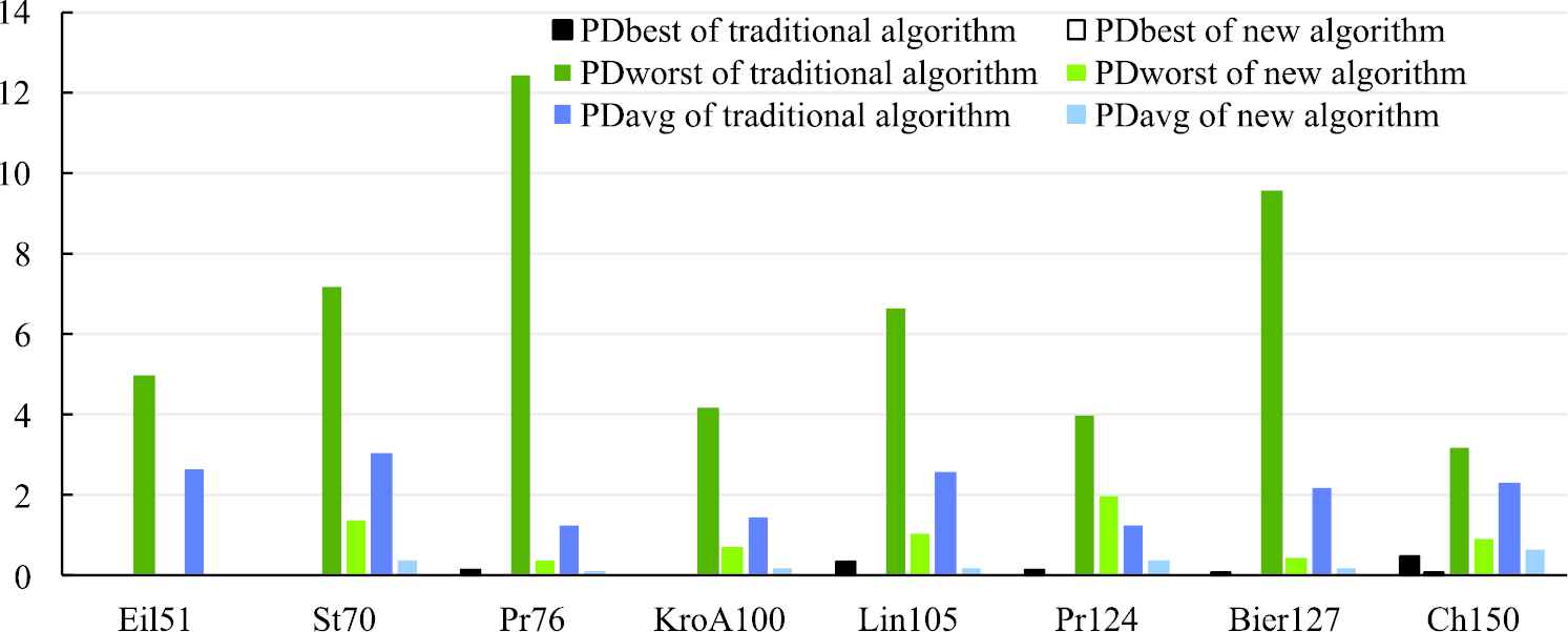
Comparison of new ant colony optimization algorithm and traditional ant colony optimization for eight TSPs.
As shown in Figure 3, for all eight TSPs, the results of the new ACO algorithm (including the best, worst, and average ones) are better than those of traditional ACO. Moreover, from Table 5, for traditional ACO, the average values of PDbest, PDworst, and PDavg are 0.14%, 6.48%, and 2.07%, respectively. In comparison, those for the new ACO algorithm are 0.0075%, 0.82%, and 0.98%, respectively. Thus, the computational relative errors of the new ACO algorithm are much smaller than those of traditional ACO. In other words, the computational precision of the new ACO algorithm is much better than that of traditional ACO. Moreover, compared with the coefficients of variation of traditional ACO, whose average value is 1.62, those of the new ACO algorithm are much smaller, with an average value of 0.98. In other words, the uniformity of the solutions of the new ACO algorithm is also much better. Therefore, the new ACO algorithm can improve the computational results and computational stability greatly for TSPs. Furthermore, compared with the results of traditional ACO, as the TSPs become more complex (greater length or more cities), the computing results are much better, and the advantages of the new ACO algorithm are better. The reason for this phenomenon may be that when the TSPs become more complex (greater length or more cities), the meeting strategy of the new ACO algorithm will be used more frequently, and thus, the increased advantage of the method of computing results in the new ACO algorithm compared with that of traditional ACO will be more noticeable.
To compare the computing speed of the two algorithms, the iterations with the best results as shown in Table 4 for the two algorithms are shown in Figure 4.
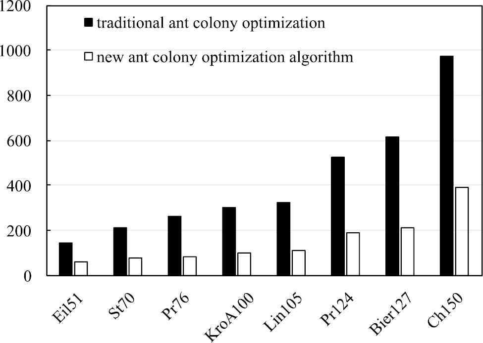
Iterations of traditional ant colony optimization and new ant colony optimization algorithm for eight TSPs.
As shown in Figure 4, for all TSPs, the computing speeds of the new ACO algorithm are all faster than those of traditional ACO. Moreover, as the number of cities increases, the difference between the computing times for the two algorithms will also increase. Therefore, as the complexity of the problem increases, the computational efficiency of the new ACO algorithm increases. In other words, the more complicated the problem, the better the computational efficiency of the new ACO algorithm.
To study the computational efficiency more comprehensively, the statistical results of the computing time for eight TSPs solved by two algorithms over 30 independent runs are shown in Table 6. In this study, two statistical indexes are used: the average computing times and the coefficient of variation for computing times. The average computing times provide information on the specific computing speed. The coefficient of variation, defined as the ratio between the standard deviation and the mean value, gives information on the uniformity of the computing speed.
| Instances | Solutions by Traditional Ant Colony Optimization |
Solutions by New Ant Colony Optimization Algorithm |
||
|---|---|---|---|---|
| Average Computing Time (s) | Coefficient of Variation | Average Computing Time (s) | Coefficient of Variation | |
| Eil51 | 12.4 | 1.21 | 7.3 | 0.88 |
| St70 | 15.6 | 1.32 | 8.8 | 0.92 |
| Pr76 | 16.7 | 1.43 | 9.2 | 0.95 |
| KroA100 | 19.3 | 1.51 | 10.4 | 1.04 |
| Lin105 | 20.1 | 1.45 | 10.7 | 0.98 |
| Pr124 | 23.7 | 1.56 | 12.1 | 1.05 |
| Bier127 | 25.1 | 1.59 | 12.5 | 1.09 |
| Ch150 | 41.4 | 1.55 | 19.7 | 1.03 |
Comparison of statistical results for computing time by the new ant colony optimization algorithm and traditional ant colony optimization for eight TSPs.
As shown in Table 6, for all eight TSPs, the computing times of the new ACO algorithm are much less than those of traditional ACO, and the coefficients of variation for the new ACO algorithm are also less. To analyze the degree of reduction of computing time by both algorithms, the reduction rate, which is the ratio of the reduction value to the computing time by traditional ACO, is obtained. For eight TSPs from Eil51 to Ch150, the reduction rates are 41.1%, 43.6%, 44.9%, 46.1%, 46.8%, 48.9%, 50.2%, and 52.4%, respectively. Therefore, as the complexity of the TSPs increases, the reduction rate of the computing time for the two algorithms also increases. Moreover, using the traditional ACO, as the scale of the TSP problem increases from 51 to 100 and 100 to 150, the corresponding computing time increases from 12.4 to 19.3 and 19.3 to 41.4, respectively. And the corresponding rates of the increasing time to the increasing scale are 0.14 and 0.44. However, for the new ACO algorithm, in the same increasing ranges of the problem scale, the corresponding computing time increases from 7.3 to 10.4 and 10.4 to 19.7, respectively. And the corresponding rates of the increasing time to the increasing scale are only 0.06 and 0.18 which are much less than those of the traditional ACO. And their rates of new algorithm to traditional ACO are 0.43 and 0.4 respectively. That is to say, the computational efficiency of the new algorithm is much high than that of traditional ACO. And as the scale of the TSP problem increases, the superiority of computational efficiency for the new algorithm will increase too. Thus, the new ACO algorithm can be used in complicated combinatorial optimization problems. The reason for this phenomenon may be that as the complexity of the TSPs (greater length or more cities) increases, the meeting strategy of the new algorithm will be used more frequently. Then, the new tour will be generated by the meeting ants quickly, and the number of new tours generated by the meeting ants will increase quickly. Therefore, the rate of increase of the computational efficiency for the new ACO algorithm will also increase.
6. CONCLUSIONS
ACO is highly suitable for performing combinatorial optimization, and is typically applied to the TSP. However, as a heuristic algorithm, it has many shortcomings, such as slow convergence speed and low searching efficiency. To overcome its shortcomings, a new ACO algorithm is proposed that enlarges the ants' search space and diversifies the searched solutions. The main strategy used in this new algorithm is to combine pairs of searching ants to increase the diversification of the solutions.
To compare the results of the new ACO algorithm with the best known solutions and the solutions found by some state-of-the-art algorithms proposed in the literature, 20 typical TSPs are used. The applications indicate that, for all the selected TSPs, the solutions obtained by the new algorithm are better than most of the other algorithms and the new algorithm is a very suitable method for solving the TSP. Finally, a comprehensive comparative study of the new ACO algorithm and traditional ACO is discussed.
Based on the above studies, the following conclusions can be drawn.
For all 20 selected TSP instances, most of the best solutions found by the new ACO algorithm are the given optimal solutions, except for seven instances. In addition, most of the average solutions found by the new ACO algorithm in 30 trials approximate the given optimal solutions, except for five instances.
The SA-SOSOA, DBA, DCSA, and the new algorithm proposed here are well-performing algorithms, and most of their best solutions are equal to the optimal solutions. Furthermore, the average solutions of those algorithms approach the optimal solutions. In fact, some of their average solutions are equal to the optimal solutions.
The results found by the new ACO algorithm are more aggregated than those found by traditional ACO. In other words, the new ACO algorithm is more stable than traditional ACO. Therefore, the new algorithm can significantly improve on the traditional algorithm.
The computing precision of the new ACO algorithm is much better than that of traditional ACO, and the computing speed of the new ACO algorithm is also faster.
As the complexity of the problem increases, the computational efficiency of the new ACO algorithm increases. In other words, the more complicated the problem, the better the computational efficiency of the new ACO algorithm.
Therefore, by comparison with traditional ACO and some state-of-the-art algorithms, the new ACO algorithm has higher computing precision, better computing stability, and faster computing speed. However, the new algorithm has only been tested on TSPs that are not very large. For large-scale TSPs, computational complexity will increase quickly, and the effect on computation may be somewhat detrimental. Therefore, comprehensive testing, especially for large-scale TSPs and for other combinatorial optimization problems, is our next task.
CONFLICT OF INTEREST
The authors declare they have no conflicts of interest.
AUTHORS' CONTRIBUTIONS
Literature search, study design, manuscript writing, data collection, data analysis, and software are all conducted by Wei Gao.
ACKNOWLEDGMENTS
This study was funded by Fundamental Research Funds for the Central Universities (grant number 2016B10214).
REFERENCES
Cite this article
TY  - JOUR
AU  - Wei Gao
PY  - 2020
DA  - 2020/01/22
TI  - New Ant Colony Optimization Algorithm for the Traveling Salesman Problem
JO  - International Journal of Computational Intelligence Systems
SP  - 44
EP  - 55
VL  - 13
IS  - 1
SN  - 1875-6883
UR  - https://doi.org/10.2991/ijcis.d.200117.001
DO  - 10.2991/ijcis.d.200117.001
ID  - Gao2020
ER  -