
RunPool: A Dynamic Pooling Layer for Convolution Neural Network
- DOI
- 10.2991/ijcis.d.200120.002How to use a DOI?
- Keywords
- Dynamic pooling; Deep learning; Malicious classification; Social network
- Abstract
Deep learning (DL) has achieved a significant performance in computer vision problems, mainly in automatic feature extraction and representation. However, it is not easy to determine the best pooling method in a different case study. For instance, experts can implement the best types of pooling in image processing cases, which might not be optimal for various tasks. Thus, it is required to keep in line with the philosophy of DL. In dynamic neural network architecture, it is not practically possible to find a proper pooling technique for the layers. It is the primary reason why various pooling cannot be applied in the dynamic and multidimensional dataset. To deal with the limitations, it needs to construct an optimal pooling method as a better option than max pooling and average pooling. Therefore, we introduce a dynamic pooling layer called RunPool to train the convolutional neural network (CNN) architecture. RunPool pooling is proposed to regularize the neural network that replaces the deterministic pooling functions. In the final section, we test the proposed pooling layer to address classification problems with online social network (OSN) dataset.
- Copyright
- © 2020 The Authors. Published by Atlantis Press SARL.
- Open Access
- This is an open access article distributed under the CC BY-NC 4.0 license (http://creativecommons.org/licenses/by-nc/4.0/).
1. INTRODUCTION
In recent years, deep learning (DL) has achieved remarkable performance in various computer applications, especially in computer vision problems [1–3]. Convolutional neural networks (CNN) is one of the popular DL algorithms for solving image recognition [4]. The architecture is based on a supervised learning model that consists of several convolutional layers and pooling layers. In neural network computation, it is required to extract more robust features against position or movement for object recognition. CNN architecture harnesses pooling layers to decrease the size of the feature map and extract features [4].
Those pooling layers are a crucial part of CNN to achieve an efficient training process. To obtain better accuracy with a small loss, subsampling plays an important role. Commonly, the CNN pooling techniques are max pooling and average pooling. In the operation process, max pooling takes the maximum score in the pooling window, and average pooling selects the average score of the pooling window. However, the current study picks pooling types without much consideration.
A paper reveals that the two conventional pooling models are not optimal [5]. In some cases, the average pooling diminishes critical information in strong activation so that it can decrease the performance on CNN. On the other hand, the max pooling shortcomings remain because it ignores all crucial information except the most significant value. It can degrade an opportunity to calculate other informative features in large and dynamic input data. A comparison with max or average pooling schemes cannot predict which parts of the input will be selected.
A paper proposes the pooling technique by replacing the conventional deterministic pooling with a stochastic model to increase pooling layer performance. It randomly selects the activation within each pooling region according to a multinomial distribution [5]. The current study introduces Deep Generalized Max Pooling that balances the contribution of all activations of a region by reweighting all descriptors [6]. Another paper proposes, alpha-pooling, which utilizes a trainable parameter α to decide the type of pooling. It is a type of pooling scheme, including max pooling and average pooling as a particular case. Demonstrated by experiment, alpha-pooling can improve the accuracy of image recognition problems. They compared several pooling layers and found that max pooling was not the optimal pooling method [7].
Besides, there are many other pooling schemes, including geometric and harmonic average. It is still challenging to find the best pooling method. Thus, it is required to keep in line with the philosophy of DL. In dynamic neural network architecture, it is not practically possible to find a proper pooling technique for the layers. It is the primary reason why various pooling cannot be applied in dynamic data problems. It needs to construct an optimal pooling method as an option of max pooling and average pooling to deal with the limitations. Not just able to select the value randomly, but also can predict which parts of the input will be selected as the most appropriate pooling value.
In this paper, we introduce a generic pooling layer as an option to construct CNN architecture. Based on our survey, it is the one pooling layer that utilizes network parameters in each layer to determine pooling value in the hidden layer. Notably, we present the main contributions of our work, particularly in CNN as follows:
We introduce a new pooling layer in the CNN architecture. Different from max and average pooling, this pooling implements a magnetic field concept in calculating the pooling layer. It runs by dynamically changing the pooling layers' values for each convolution in the hidden layer.
We construct the pooling layer by obtaining several hyperparameter in each layer. Then, this function calculates the parameters with a range distribution. By establishing the concept, we get the state-of-the-art in CNN architecture. By demonstrating the architecture, we harvest higher accuracy and a smaller loss than conventional CNN architecture max pooling and average pooling layer.
Notably, this function is different from traditional pooling that obtains the highest valued activation out of the pooling window or takes an average value of a pooling window. The proposed pooling layers try to find appropriate pooling value to achieve efficient computation by calculating several informative parameters in each layer. It is a novel pooling approach in CNN architecture to reduce overfitting while training a model.
The rest of the paper is structured as follows: Section II gives insight into the proposed technique, Section III presents the experimental setup that consists of case study in a social network, dataset, and data preprocessing. Section IV describes the result and discussion. Section V offers the conclusion and highlights some open research questions in CNN architecture.
2. PROPOSED TECHNIQUE
As the hot topic of research, DL is becoming an increasingly popular approach for solving diverse applications. The CNN algorithms imitate the structure and function of the human brain [8]. In recent years, CNN has achieved state-of-the-art results on a variety of challenging problems in computer vision and speech recognition. Research communities have implemented this concept to deal with many computer assignments. Several papers explore the use of deep belief networks (DBN) for authorship verification by a Gaussian–Bernoulli in DBN [9], face verification with a Deep Neural Network (DNN) [10], and document recognition [11].
2.1. Convolutional Neural Network
Most of the current research in DL propose CNN architecture to deal with various problems, including image, voice, video, and object detection [8]. In this paper, we construct a CNN architecture by adding a new pooling layer in the neural network. We mention the graph as dynamic CNN, a CNN graph with a RunPool pooling function that has three layers in the network, including an input layer, a hidden layer, and an output layer. In the input layer, the network layer projects the feature extraction as matrices input. To compute the feature extraction result, we adopt convolution layer processing with weight sharing. Thus, it is unnecessary to optimize many parameters because the method can construct convergence faster.
This architecture adopts the convolution to address multiple input feature maps and to produce stacked feature maps of increasing layers. In this experiment, we define a feature map of
The model defines the computation of the convolution process between filters and input matrices. The model convolves a set of filters form
After convolution operation, we construct a pooling layer to obtain the most informative values in the hidden units. Pooling aims to convert the joint feature representation into a more valuable point that preserves important information and diminishing irrelevant details. In operation, the pooling reduces the resolution of the feature maps over the local neighborhood of the previous layer. Commonly, a CNN architecture employs conventional pooling schemes such as max pooling and average pooling to obtain a maximum or average value in the hidden layer. The max pooling chooses the biggest element in each pooling region as:
On the average pooling function,
In some image recognition problems, both the max pooling and average pooling have their shortcomings. Figure 1 illustrates the drawbacks of max pooling and average pooling in detecting a diagonal line.

Pooling process of input feature that illustrates the drawbacks of max pooling and average pooling on CNN.
In the pooling region, max pooling only considers the maximum element and ignores others. In some cases, it will lead to an unacceptable result because if the most elements consist of high magnitudes, the distinguishing feature vanishes after max pooling. On the other hand, the average pooling gets worse if there are many zero elements on the input features; the characteristic of the feature map will be reduced largely [12].
Therefore, as a new way to downsampling the features, we consider replacing the deterministic pooling function with a stochastic scheme. Instead of using the standard pooling method, we introduce a new pooling function by adopting a nondeterministic pooling concept.
2.2. Main Idea
To construct a pooling function with a stochastic pooling paradigm, we take a magnetic field problem as the basic idea. The main problem of this function is how to establish a CNN architecture by optimizing a new pooling layer. We are inspired by a model that adopts the dynamic k-max pooling to compute the engineered feature in each layer. By choosing the hyperparameters in each layer, the function calculates the pooling value to obtain a pooling sequence in 1D dataset [13].
To implement the magnetic field concept, we calculate the pooling layer with the Gaussian Law theory (Gaussian random variable). At the initial step, we compute the pooling function by generating random numbers from a Gaussian distribution. We employ the random technique because the randomness comes from atmospheric noise. In several computer applications, it is better than the common pseudo-random algorithms. A normal distribution has a bell-shaped density curve described by its mean
In formula 2,
2.3. RunPool Pooling
CNN is a famous DL architecture that uses a lot of identical copies of the same neuron. The process runs extensive computation with a little number of parameters and has many interleaved convolutional and pooling layers over the network. The CNN layer receives a single input (the feature maps) and computes feature maps as its output by convolving filters across the feature maps. CNN can ignore the aspect of feature engineering with automatic representation.
One critical layer in CNN training is the pooling layer. The pooling can act as a generalizer of the lower-level data in the NN training. It is a sliding window technique that utilizes several kinds of statistical functions to get the contents on each window. There are two common types of pooling techniques, max pooling and average pooling. Max pooling employs the max function to obtain informative materials, while the average pooling harnesses the statistical mean function to take the contents of the window. Principally, a pooling function simplifies the output features by performing nonlinear computation and reducing the number of parameters.
Instead of using the conventional pooling layers, we construct a method that dynamically changes the pooling values based on the current network parameter. It takes the length of the input vector of the network to obtain a feature map according to the current parameters in each layer. The basic idea of the function is how to calculate network elements of the current map pooling and to find appropriate pooling value by comparing it with a constant pooling value. It is to recompute the pooling value using the layer parameters and learn a CNN hierarchy of feature orders. Figure 2 depicts the CNN computation with the RunPool pooling layer in the visible and the hidden layer.
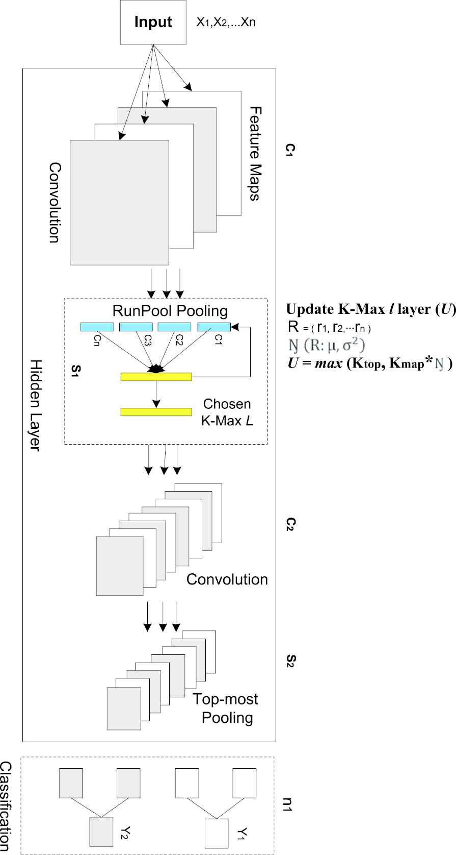
The network topology of proposed CNN with input
The hidden layer runs the convolution process by using filters and input matrix. In the model, a set of filters form
| Notation | Description |
|---|---|
| f | Filter size |
| s | Stride |
| l | Index of the current layer |
| k value of the current layer | |
| k value of the top layer | |
| k value after calculation of input features | |
| L | Total number of layers |
| C | Length of input vector (sequence of features) |
| p | Padding |
Mathematical notation of RunPool pooling algorithm.
We construct the function to allow a smooth extraction of higher order and to adapt with a longer range element at the hidden layer. The model employs the k value at intermediate layers (hidden layer). The dynamic CNN calculates forward pass with the following function.
In the above formula, the first network computes the features maps as the input layer to the CNN. In Equation (4),
In the backward pass process with Equation (6), the layer will compute the gradient of the l (loss function) with respect to
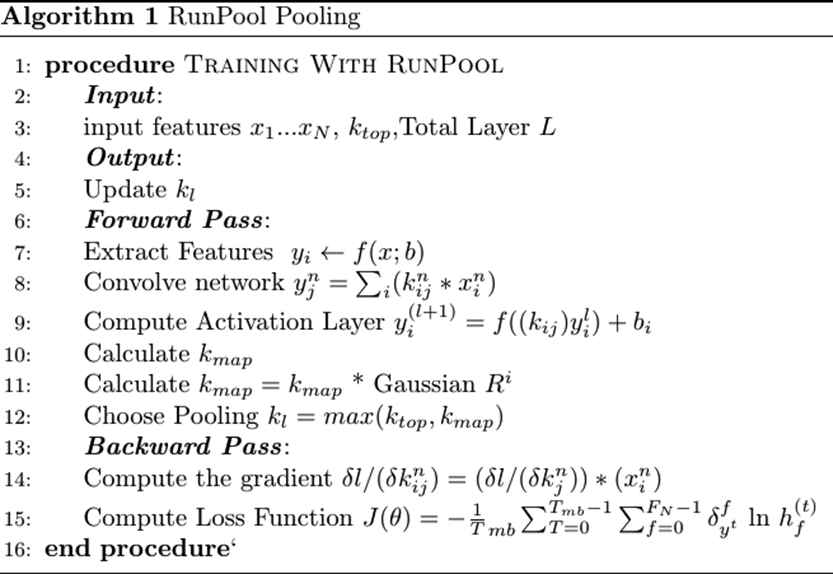
RunPool Function: Assume k be a function of the length of the input and the depth of the network as the computing model. l is a current convolution in the hidden layer, L is the total number of convolution layer. At the initial process, we determine ktop as a constant value for the pooling layer calculation. The function needs input matrices and some padding to calculate the extracted features. It computes
In CNN process, each convolutional filter produces a matrix of hidden variables. The pooling layer is utilized to reduce the size of the matrix. Max pooling is a procedure that takes an
Pooling layers are a downsampling layer that combines the output of layer to a single neuron. The model calculates the input data in the hidden layer with
Inspired by DCNN model in [13] with one-dimensional convolution, we construct a function to obtain appropriate k-max pooling value by using more layer parameters with dynamic values. Then, we take Gauss distribution to calculate the final
From the function above, the RunPool selects
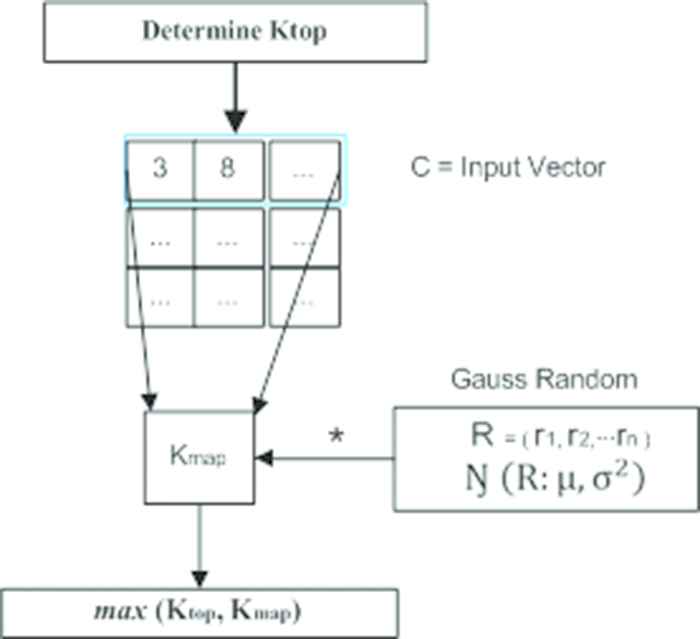
Obtaining a pooling value by using RunPool function in the proposed CNN. The proposed CNN computes the input dinput = x1, x1, ‥ xn and some window parameter dlayer to get kmap. At the final step, it compares ktop constant and obtained kvalue to take the pooling value.
The main idea of the function is how to take some parameters of the current layer to obtain appropriate pooling value in the current hidden layer. In the RunPool function, l is some current convolution in the hidden layer, L is the total number of convolution layer, ktop is the fixed max pooling parameter for the topmost convolutional layer. To obtain optimal max pooling value, we calculate the RunPool function with Algorithm 1.
Algorithm 1 describes how to calculate the network parameters to take
We activate the pooling function between the convolution and before the fully connected layer (FC). FC is an efficient way of learning nonlinear combinations to classify the data into target (categories)
For calculating error loss of the model, the experiment utilizes cross-entropy (CE) loss function. We calculate the loss function with the function:
The above criterion function consists of
3. EXPERIMENTAL SETUP
In this study, we experiment with a large amount of 1D datasets, including numerical and text datasets. We gather a large dataset to construct a benchmark sample for the training and testing model with the dataset. In this paper, we focus on the 1D dataset, including texts, characters, and numeric data, to measure the pooling performance in training the model.
3.1. OSN Classification
In this experiment, we collect a large online social network (OSN) as the primary dataset and train it as a binary classification problem. OSN is a large environment with a large amount of data with millions of users. OSN become a popular application for sharing a lot of data items including videos, photos, and messages. The main trait of OSN is the social relation. It contains a large number of accounts. They post, send, and share any data items across the platforms. Indeed, it is easy to gather much information across the sphere. OSN is a dense interconnection among the user of the network. In reality, OSN's model is mostly multirelational that contains a large number of nodes. Basically, in the research area, the OSN depicts the nodes by a graph. The nodes represent actors who build diverse relationship type edges that reflect actor interactions [14]. In current years, OSN becomes an active research interest in several fields [15].
In the OSN environment, analyzing the data characteristic can produce patterns of knowledge of the underlying OSN activities and hidden regularities. Link prediction, as one of the hot topics in social network research and as one of the analysis problems since a decade, drives a big amount of the researcher's attention from various disciplines [16]. However, the OSN environment remains as security issues and become the primary concern in the fast-growing OSN. Protection technique is one of the most critical aspects of an (OSN). The shortcomings of security and privacy-preserving model put the user data at risk. Many papers propose various techniques to address the OSN security issue [17,18].
Commonly, the OSN system conducts anomaly detection by monitoring a sudden user discrepancies activity. If the users' activities keep on changing in a period abruptly, the OSN provider catches the suspicious account up by the changing of access pattern. If it fails to gain the information and behave with unusual pattern, the abnormal can infect the system with existing fraudulent [19]. However, suspicious activity exhibits different patterns, type of data, level of interaction, and the difference in time usage. To identify the anomalies, it needs to classify in detail the features of users. In this paper, we focus on building a classification model with supervised learning by computing the OSN dataset in the training process.
3.2. Dataset
In this experiment, we provide the OSN dataset as a 1D dataset and feed the features into the supervised learning algorithm. At the first stage, we collect the OSN dataset consists of some high-level features of OSN, such as user profiles
In this paper, we define OSN as G and is represented by
OSN graph
3.2.1. OSN link features
Current research discusses various DL methods to conduct link prediction [20,21]. In the OSN communities, anomalies link become one of the primary concerns of OSN security research. Initially, the source of menace comes from suspicious user activities. The infected user automatically spread fake information or deceive user for targeting other regular users. If the crumbly system cannot adopt the threat model, it becomes an easy target for phishing or compromising attack. An anomaly has a diverse type of threat like vertical attack and horizontal attack. A vertical is usually a threat to the providers, and the horizontal one poses attacks to other OSN users [22].
The current study discusses fake account detection in social networks by using the learning method. DeepScan proposes malicious account detection with DL in Location-Based Social Networks (LBSN) [23]. Another scheme utilizes the similarity of the user's friends to calculate the adjacency matrix of the graph to identify the user as benign or fake [24]. Analyzing social relations is a new way of determining anomalous users by mapping social ties and geographical among users. It calculates OSN factors like friendship, common interest, or alliance to determine chosen friends. Many researchers have proposed methods to construct the OSN security model. Therefore, in this paper, we build a learning classifier as a new way of protection by analyzing the OSN dataset.
We gather the OSN link dataset of the OSN from several public OSN, especially the undirected OSN graph. In the security case, link prediction is a crucial part of analyzing the structure in the OSN as a security scheme. Instead of exploring the entire graph, we gather the neighborhood link information by aggregating the features. For this experiment, we collect topology information of the network which is available from the data domain. We gather the undirected OSN dataset from Facebook and Flickr samples to build the benchmark dataset. Table 2 displays the dataset which is gathered for the experiment.
| Properties | Facebook Dataset | Flickr Dataset |
|---|---|---|
| Size | 63,731 vertices (users) | 1,715,255 vertices (users) |
| Volume | 817,035 edges (friendships) | 15,551,250 edges (links) |
| Average degree | 25.640 edges / vertex | 18.133 edges / vertex |
| Size of LCC | 63,731 vertices (users) | 1,624,991 vertices (users) |
| Gini coefficient | 64.3% | 88.2% |
| Relative edge distribution entropy | 93.1% | 82.2% |
| Assortativity | 0.17702 | –0.015282 |
| Clustering coefficient | 14.8% | 11.2% |
LCC, Largest Connected Component.
Dataset of link prediction and classification.
This corpus contains the undirected network link of OSN users. In the dataset, a node denotes a user, and an edge indicates a friendship between two users. The datasets contain a subset sample of the total friendship graph. Notably, measuring social relation with supervised learning such as CNN becomes a new approach in OSN malicious link detection. The main problem of node relation analysis is to quantify links among the user and classify the user categories. Finally, we feed the sample into the learning model to train the OSN attributes (user relations and profiles features) to classify the OSN account.
3.2.2. OSN profile features
In this part, we gather OSN user-profiles information as the experiment dataset that contains many features that can be trained for building a classification model. The public OSN usually obtain the attributes for computing purposes. It is a way to handle the user and activity anomalies problem. Activity variations among accounts with contrast behavior from different OSN groups cause horizontal anomalies [25]. Thus, we take advantage of the vast user information as the sample to construct an effective learning model as the OSN protection.
Firstly, we define OSN as G and is represented by
In this study, we provide sample OSN profiles with more than 3000 unique users. We build a dataset by decomposing some user profiles information. For the experiment dataset, the paper observes user data around 3000 OSN members. We provide 1500 data with a normal user profile and 1500 users with fake profiles label. We split the training data and testing dataset to achieve real accuracy and loss.
3.3. Data Preprocessing
The aim of data preprocessing is to convert the raw dataset at hand to the input vector for NN training. At the preprocessing, we separate the several features into parts to preserve the context of each token. A feature gets a different value when is extracted from the identity, hostname, location, time, and other attributes of OSN. The stage includes vectorization, normalization, handling missing values, and feature extraction.
In the data preprocessing, we split the dataset into a training and test part. For training the model, we employ the training data and evaluate the model on the validation data. After finishing the validation model, we test the final model on the test data. For testing the model, we need to use a wholly different and unseen dataset to evaluate the model with the test dataset. We set the model to be unable to gain access to any information about the test dataset.
This study suffers from a not balanced dataset because the data contains about 90%–95% that belong to the same majority class (benign account). If we conduct training on such data, it can cause the ignorance of the clarification of minority clusters (fake account). Thus, it can influence the overall accuracy of classifications. To deal with this issue, we utilize the Synthetic Minority Oversampling Technique (SMOTE) to balance the dataset [26]. It is a relevant approach if we want to obtain the similarity feature of the nodes and avoid to diminish information.
In the initial prepreprocessing, we utilize a function to convert integer and string dataset into the input matrix. We need the technique to convert the features into a vector because the input may be an array of data like integers or strings that cannot be processed in neural network training. In the final phase of preprocessing, we separate the dataset into training and testing datasets to test the model on unseen data. We have two labels for the evaluation dataset, and these are benign and malicious targets.
We feed a few noises data to make it difficult for the model to be bias-free and reflects a real condition in a classification problem. Thus, the model will consider the noisy data patterns, and it pushes the model toward overfitting in the training and testing process. After the preprocessing stage, the model feeds the features into the graph for classification. To train the model, we feed the dataset into the proposed CNN to make predictions on new unseen data with binary classification tasks.
4. EXPERIMENT RESULT
Based on the experimental setup, we have conducted training and testing by gathering two groups of OSN dataset. In this section, we have shown how the generic pooling layer's performance in link classification and fake profile detection in the benchmark OSN dataset. In this part, we have displayed the accuracy and loss of the pooling scheme. The experiment also has provided an evaluation of the performance model by using cross-validation. It is to calculate Recall, Precision, F1 Score, Receiver Operating Characteristic (ROC) [27].
4.1. OSN Link Classification
In the link prediction problem, we have gained a trade-off between the accuracy and the performance time. By tuning diverse hyperparameters, we have undergone the neural network performance. In the training and testing process, we have tuned epoch = 500, batch size = 50, and with learning rate (lr = 0.01). Table 3 describes the proposed CNN performance, especially in the training and testing process.
| Input | Hyperparameter | Optimizer | Training Loss | Testing Loss |
|---|---|---|---|---|
| FB link | Adam | 0.5033 | 0.5069 | |
| #50000 | Dropout p = 0.6 | SGD, m = 0.5 | 0.5068 | 0.5070 |
| H1 = 64 | ||||
| H2 = 32 | ||||
| Adagrad | 0.5057 | 0.5059 | ||
| RMSProp | 0.5176 | 0.5223 | ||
| Flickr | Dropout p = 0.6 | Adam | 0.5052 | 0.5060 |
| #50000 | H1 = 64 | |||
| H2 = 32 | ||||
| SGD, m = 0.5 | 0.5178 | 0.5160 | ||
| Adagrad | 0.5075 | 0.5074 | ||
| RMSProp | 0.5092 | 0.5087 |
FB, Facebook.
CNN with RunPool layer performance in link classification with different parameter setting.
We have tested gradient descent and tune optimization algorithms with different hyperparameters by computing this sample. We have employed the gradient descent to minimize the objective function
Moreover, we have tested RunPool CNN with another gradient descent like stochastic gradient descent SGD with a momentum that also produces a competitive result. The SGD with momentum (m = 0.5) can provide a better result if we tune in larger epoch and big regulizer. However, the experiment has found that adding more hidden layers for SGD cannot reduce the loss. Using a large number of hidden layers has caused overhead computation in a particular device, especially in CPU processing. Testing the NN by adding more layers and neuron numbers of CNN could not engage in improving the predictive capability. Because of the limitation of neuron number, it enlarges computing resources. Thus, using the RunPool pooling function can increase the accuracy result without adding more hidden layers in a neural network.
In this experiment, we also calculate the Recall function to define the percentage of the datasets that belong to the malicious and identifies it as malicious. The precision determines the rate of the datasets which identifies as malicious, but actually, do not include the malicious. Finally, we want to seek a balance between Precision and Recall. We need to measure the OSN account classification who have the malicious link by accepting a low precision if the testing result is not significant. Hence, we require an F1 score as an optimal blend of Precision and Recall. Tables 4 and 5 show the Recall, Precision, and F1 Score in both OSN datasets.
| Classification Model | Accuracy | Average Precision and Recall | F1 Score |
|---|---|---|---|
| Bernoulli | 78.77 | 0.2123 | - |
| Logistic regression | 91.49 | 0.6803 | 0.7563 |
| SVM (rs = 40) | 91.95 | 0.6974 | 0.7724 |
| SVM (rs = 50) | 91.99 | 0.6990 | 0.7745 |
| S-neural network | 94.10 | 0.9120 | 0.9210 |
| Proposed approach | 98.04 | 0.9775 | 0.9595 |
Accuracy and F1 Score with several machine learning algorithms for the Facebook dataset.
| Classification Model | Accuracy | Average Precision and Recall | F1 Score |
|---|---|---|---|
| Bernoulli | 78.77 | 0.2123 | - |
| Logistic regression | 92.06 | 0.7048 | 0.7787 |
| SVM (rs = 40) | 92.47 | 0.7217 | 0.7897 |
| SVM (rs = 50) | 92.52 | 0.7257 | 0.7938 |
| S-Neural network | 94.10 | 0.9280 | 0.9321 |
| Proposed approach | 98.34 | 0.9732 | 0.9846 |
Accuracy and F1 Score with several machine learning algorithms for the Flickr dataset.
Based on the table above, the accuracy result has shown that supervised machine learning produces different accuracy. There are Naïve Bayes (78.77%), Logistic Regression (LR) (92.06%), Support Vector Machine (SVM) (92.47%, 92.52%), and Neural Network (NN) (94.10%). The proposed CNN architecture with the RunPool layer can produce about 98.34% in several times of the testing process with the benchmark dataset. To make sure the model performance, we add a few noise data into the dataset that makes the common Machine Learning (ML) algorithm more difficult to make a classification. Fortunately, the proposed CNN can achieve better accuracy than other ML algorithms. We also calculate the Area Under the Curve (AUC) score that produces the highest score of the AUC = 0.9970. It reflects that this model can achieve a good level of prediction in the classification problem.
4.2. OSN Account Classification
In this section, we test the proposed RunPool with several learning parameters to classify the user categories based on OSN profile attributes. In the training process, this study was tested with some popular optimizers, including SGD with momentum, Adam, Adagrad, and RMSprop. The study calculates the gradient of loss when training networks in the critical part to measure comparison result between training and test result. We have put the local variable concept to compute the loss function and compute the gradient of the loss concerning the weight with various learning rates.
In this experiment, we tune the gradient descent and optimization algorithms with different hyperparameters. In NN training, choosing the value of a hyperparameter is one of the most important parts to increase the network training quality. By tuning appropriate hyperparameters in the CNN, we obtain the highest performance of the neural network. In the training and testing process, we tune epoch = 15 and batch size = 50. We have produced a trade-off between the accuracy and the performance time. Table 6 describes the proposed CNN performance in computing validation accuracy and loss.
| Parameter | Optimizer | Val-Loss | Val-Accuracy |
|---|---|---|---|
| Dropout p = 0.5 | Adam | 0.3633 | 0.9131 |
| H1 = 32 | SGD, m = 0.9 | 0.2087 | 0.9291 |
| H2 = 64 | Adagrad | 0.3620 | 0.9025 |
| RMSProp | 0.4049 | 0.8794 | |
| Dropout p = 0.3 | Adam | 0.4018 | 0.8954 |
| H1 = 16 | SGD, m = 0.9 | 0.2143 | 0.9344 |
| H2 = 32 | Adagrad | 0.3559 | 0.8989 |
| RMSProp | 0.4017 | 0.8865 |
Classification result of the proposed CNN with RunPool layer in with different parameter setting.
This experiment also tests the Precision, Recall, and F1 Score to compare how significant the impact of the proposed pooling layer in classification assignment. Table 7 shows the Recall, Precision, and F1 Score with different algorithms.
| Classification Model | Precision | Recall | F1 Score |
|---|---|---|---|
| Bernoulli (Naïve Bayes) | 86.90 | 86.94 | 87.00 |
| Gradient Boosting (n estim=50) | 90.66 | 90.69 | 91.00 |
| Logistic Regression | 90.47 | 90.59 | 90.61 |
| SVM (rs = 31.6) | 90.04 | 87.34 | 87.24 |
| S-Neural Network | 92.10 | 92.80 | 92.91 |
| Proposed Approach | 94.00 | 93.21 | 93.42 |
Comparison result between some common classification algorithms and the proposed approach in the OSN dataset.
Based on the table above, accuracy result has shown that supervised machine learning produces diverse accuracy. There are Bernoulli Naïve Bayes (86.90%), Gradient Boosting (GB) (90.66%), LR (90.49%), SVM (90.04%), NN (92.10%). The proposed CNN architecture with the RunPool pooling layer can produce 94.00% in several times of the testing process with the benchmark dataset. We have found that the proposed pooling layer can harvest the highest accuracy than other common machine learning in the benchmark OSN user-profiles dataset. At the final stage, we also calculate the ROC curve as a binary classification. The ROC curve shows that the proposed model can produce an AUC area of more than 0.9. It reflects the model that it can be a good classifier for training the dynamic dataset such as OSN.
4.3. Pooling Comparison
In this part, we provide the comparison result among RunPool Pooling, Max Pooling, and Average Pooling to calculate model accuracy. We calculate the accuracy of the model combined with different pooling functions to measure the performance of each pooling in the classification task. This study tested the accuracy among RunPool Pooling, Max Pooling, and Average Pooling in the same hyperparameter tuning and environment. It is to convince the performance of each pooling in the classification task. Table 8 displays a comparison result among different pooling function by using 2254 training samples and 545 validation samples.
| Pooling Type | Epoch = 7 | Epoch = 10 | Epoch = 15 |
|---|---|---|---|
| Average Pooling | 91.13% | 91.49% | 87.94% |
| Max Pooling | 91.21% | 91.31% | 89.89% |
| Max. Pool + RunPool | 91.67% | 91.67% | 89.36% |
| Avg. Pool + RunPool | 91.40% | 91.89% | 88.48% |
| RunPool Pooling | 92.38% | 92.54% | 91.08% |
Comparison of validation accuracy among pooling functions when training with the same hyperparameter tuning and dataset.
In the first experiment, the study trains the classifier without a pooling layer that means CNN replaces the pooling layer by convolution with stride. However, CNN without pooling cannot produce a good result in diverse training periods. In this case, CNN requires pooling layers to reduce the dimensions of output features and render some amount of invariance. Based on the training result, CNN with pooling layers are better than without pooling.
To ensure the performance among RunPool Pooling, Max Pooling, and Average Pooling, we add the pooling layers into the CNN. As we know, Max Pooling and Average Pooling are deterministic pooling types that take the pooling value upon the maximum and average score of a pooling window. Instead of using ordinary deterministic pooling, we test the RunPool as a nondeterministic pooling to train the CNN model in the classification task. The experiment shows that the proposed CNN with RunPool Pooling can achieve a promising accuracy for an account classification task. However, this experiment suffers from decreasing accuracy when trained with a large epoch (many iterations). It can be solved by providing more dataset for training the model.
At the final stage, we evaluate the classifier by using ROC and AUC scores. This technique is used to assess the false alerts of malicious detection. Based on the experiment, the graph depicts a comparison among several pooling layers in calculating the AUC score and False Positive Rate (FPR) score. Figure 5 depicts the AUC comparison among three pooling functions in malicious classification by using OSN features as the dataset.

Comparison result of the AUC score among Max Pooling, Average Pooling, and RunPool Pooling layer in the malicious classification task.
Figure 4 depicts that the AUC scores with the proposed approach (a) are higher than the conventional pooling layer (a) and (b). In this part, we plot AUC as a binary classification by adopting problem distributed observations
To sum up the benefit of the proposed pooling layer in the CNN architecture with the 1D dataset, we have presented the training and validation result by calculating the huge sample (OSN features). We find that the proposed CNN with RunPool can achieve an efficient result and increase the learning performance of the neural network. In DL study, the proposed pooling technique can be an alternative way to train a DL model not only for the 1D dataset (text) but also for a 2D dataset (image) and 3D dataset (video and voice).
5. CONCLUSION
In this paper, we introduce a new pooling layer called RunPool to find different optimal pooling values within the pooling window. We propose the pooling function to deal with deterministic pooling issues by harnessing some network parameters to obtain an informative feature map. It calculates some layer parameters and Gaussian distribution numbers based on
In the test process, we obtain a dynamic optimizer that is better to achieve high accuracy and small loss. On the other hand, the SGD with momentum also produces a competitive result. It can provide an accurate and minimum loss if we tune it with a larger epoch and big regulizer. SGD with momentum optimizer become an excellent option to train the CNN RunPool model. In fake OSN account classification, we compare the proposed CNN accuracy to the supervised ML, including Bernoulli Naïve Bayes (86.90%), GB (90.66%), LR (90.49%), and SVM (90.04%). The proposed CNN can achieve the highest score by producing 94.00%.
Demonstrated by experiment with 1D OSN dataset, it is confirmed that RunPool can improve the performance of the CNN to address the drawback of common max pooling and average pooling. This type of stochastic pooling can be combined with the common pooling layers to produce better accuracy with tiny loss. By implementing CNN with RunPool, we harvest an increased level in the graph's performance and gain better accuracy in the validation process for the classification case. Not just calculate the accuracy and loss, we also conduct the evaluation metric to measure the performance of the classifier. By calculating the Precision, Recall, and F1 Score, we obtain a promising result because the proposed model can achieve the highest AUC score.
As the future directions of malicious classification study with DL, it needs an exploration for handling accounts and malware hierarchy links that reflect the source of the threat. Then, neural network computation is necessary to calculate with a new technique like adaptive loss function rather than a regular loss function. We also suggest the next study to test this model by utilizing a 2D dataset (image) and 3D (video or audio) dataset for measuring training and testing accuracy.
CONFLICT OF INTEREST
The authors declare they have no conflicts of interest.
AUTHORS' CONTRIBUTIONS
All authors has contribution in this research.
ACKNOWLEDGMENTS
This paper is conducted in the Institute of Research in Information Processing Laboratory, Harbin University of Science and Technology under CSC Scholarship (No. 2016BSZ263). This project is available on Github.
REFERENCES
Cite this article
TY  - JOUR
AU  - Huang Jin Jie
AU  - Putra Wanda
PY  - 2020
DA  - 2020/01/28
TI  - RunPool: A Dynamic Pooling Layer for Convolution Neural Network
JO  - International Journal of Computational Intelligence Systems
SP  - 66
EP  - 76
VL  - 13
IS  - 1
SN  - 1875-6883
UR  - https://doi.org/10.2991/ijcis.d.200120.002
DO  - 10.2991/ijcis.d.200120.002
ID  - Jie2020
ER  -