
Using Recurrent Neural Networks for Part-of-Speech Tagging and Subject and Predicate Classification in a Sentence
 , Luis Rodriguez-Benitez, Luis Jimenez-Linares, Juan Moreno-Garcia*,
 - DOI
- 10.2991/ijcis.d.200527.005How to use a DOI?
- Keywords
- Natural language processing; Part-of-speech (POS) tagging; Recurrent neural networks; Syntactic analysis
- Abstract
In natural language processing the use of deep learning techniques is very common. In this paper, a technique to identify the subject and predicate in a sentence is introduced. To achieve this, the proposed technique completes POS tagging identifying in a later stage the subject and the predicate in a sentence. Two different deep neural networks are used to complete this process. A first one to establish a correspondence between individual words and part-of-speech (POS) tags and a second one that, taking as input these tags, identifies relevant elements of the sentence such like the subject and the predicate. To validate the architecture of our proposal a set of tests over public datasets have been designed. In these experiments, this model achieves high rates of accuracy in POS tagging and in subject and predicate classification. Finally, a comparison of the results obtained for each individual network with similar tools such as NLTK, pyStatParser and spaCy is made.
- Copyright
- © 2020 The Authors. Published by Atlantis Press SARL.
- Open Access
- This is an open access article distributed under the CC BY-NC 4.0 license (http://creativecommons.org/licenses/by-nc/4.0/).
1. INTRODUCTION
Analysis of written texts in natural language is more and more frequently allowing to extract information from them. This research line is known as “natural language processing” (NLP) and currently intensive research is related to it. Specially, it is intended that a machine would be able to understand the natural language from different sources (image, sound or text) [1]. NLP is a part of artificial intelligence and deals with the generation and processing of natural language. NLP is the set of techniques for automatic analysis and representation of human language. NLP has undergone a great change since it began reaching the ability to process millions of web pages in less than a second [2]. NLP allows operations related to natural language at all levels, for example, computations related to parsing and part-of-speech (POS) tagging or machine translation and dialogue systems.
A text in natural language is composed using a set of grammar rules [3]. Therefore, the texts are broken down into sentences for its processing. A sentence is a set of words that are formed following a set of syntactic rules. In addition, words are constructed using formation rules. The meaning attributed to each word along with the syntactic construction that organizes its appearance in a sentence is needed to understand the text. Then, to interpret natural language it is required the analysis of lexical, syntactic and semantic information available in a text. It can be said that in natural language the sequence is more important than individual elements, therefore, deep neural networks (DNNs) are a good tool to process natural language. Today many of the NLP techniques are based on language models produced by machine learning and techniques based on DNN are very frequent. For example, these types of networks are frequently used in sequence labelling, NLP and text classification. Young et al. [4] present a significant number of deep learning-related models that have been used for NLP tasks showing their evolution in recent years.
In real applications it is needed to extract information from text written in natural language [5–7]. For example, online shopping has customer reviews about products and services that need to be automatically interpreted and labelled so that users can easily access the information [8,9]. Sentiment analysis can be an example of this because it decides if the consumer or client has a positive or a negative opinion about a product or service [10,11]. Therefore, the development of tools that allow an automated analysis of all this information is an important research field. Within this research field, the detection of the different phrases that make up the sentence can help in the performance of that analysis since each phrase is associated with a specific function within the sentence, which is an outstanding information to be used in order to classify and label it.
This document deepens in the detection of the subject and predicate as first step for the detection of the phrases of the sentence being this the key to perform the automated analysis of information in natural language. By means of the use of DNNs, the proposed technique completes POS tagging and later identifies the subject and the predicate in a sentence. Two different DNNs are used to achieve this. We decided to focus on a model based on a Bidirectional-LSTM neural network. The model is able to perform POS tagging and subject and predicate classification. To do so, two different neural networks have been used. The first one is in charge of classifying the words with the POS tags. With the second one, the POS tags from the first network are used to identify the subject and predicate of the sentence. This model achieves 90.38% accuracy in POS tagging and 91.74% in subject and predicate classification. The results obtained with each network improves the results obtained with other tools that we have used to compare with, tools like NLTK and pyStatParser [12].
The rest of this paper is organized as follows: Section 2 presents relevant research related to NLP and DNNs applied to natural language. Section 3 details a description of the architecture of the designed neural network to carry out the syntactic analysis. Section 4 exposes the preprocessing needed to adapt the input sentences to the network structure. Section 5 presents the obtained results from the tests. Finally, in Section 6, some conclusions is indicated.
2. BACKGROUND
DNN are being used very frequently to solve tasks related to NLP. These techniques have undergone a great evolution over time. Statistical NLP is one of the most used tools for processing and generation of natural language. In its beginning, it presented problems in learning the joint probability functions of language models due to dimensionality. For this reason, distributed representations of existing words in a low-dimensional space began to be used [13]. Among these techniques word embeddings, also called distributional vectors stand out. Word embeddings are based on the fact that in a given context there are words with similar meaning (distributional hypothesis). Vectors store the characteristics of their neighbors. Subsequently, the similarity between these vectors can be measured using similarity measures. Word embeddings are often used as the first layer of data processing in a deep learning model [4]. In 2013 Mikolov et al. [14,15] introduced an improvement of word embeddings known as Continuous Bag of Words (CBOW) and skip-gram models. CBOW relies on a window mechanism of size k to calculate the conditional probability of a target word given the context words surrounding it. The skip-gram model predicts the surrounding context words given the target word. Morphological and intra-word information can also be very useful for tasks such as POS-tagging and Named-Entity Recognition (NER ). There are some publications related to the construction of natural language comprehension systems at the character level [16,17]. Another possibility is known as “character embeddings” and other set of techniques make use of Convolutional Neural Networks (CNNs). These networks have been used in NLP to obtain functions that extract higher level features than words (n-grams) [18,19] that are used in various NLP tasks such as sentiment analysis, summarization, machine translation and question answering (QA).
Collobert and Weston were the first ones using CNN to model sentences [18]. This work used multi-task learning to generate multiple predictions for POS tags, chunks, named-entity tags, semantic roles, semantically-similar words and a language model. Its operation is based on obtaining a vector of user-defined dimensions that represents a word from a look-up table. Subsequently Collobert [19] proposed a general framework based on CNN to solve NLP tasks which marked the beginning of the use of CNN for NLP. Another of the first publications that uses CNN for NLP tasks was proposed by Kalchbrenner et al. [20] and Kim [21]. A window approach like the one mentioned above was also proposed to be able to make predictions based on words that are necessary in tasks such as NER, POS tagging and Semantic Role Labeling (SRL). A multi-level deep CNN have demonstrated their proper operation to label each word in a sentence as a possible aspect or nonaspect. Poria et al. [22] achieved outstanding results in the aspects detection. The conditional random field (CRF) has allowed the dependencies between adjacent class labels to be obtained by creating a coherent sequence of tags. This sequence allows the complete sentence to reach a great score at the word-level classification [23]. Young et al. [4] detail some relevant works of literature that use CNN for NLP tasks.
Recurrent Neural Networks (RNNs) have also been frequently used to solve NLP tasks. These networks process the input information sequentially, that is, they perform the same calculation for each token in the sequence considering the previous results, so it is said that the RNN have memory [4]. There exist several kinds of recurrent neural networks that have been proposed in the literature. Basically, they try to mitigate some of the inherent problems that underlies the error propagation method, as well as the complexity of these networks. In this sense, the [24] Long Short Time Memory (LSTM) and the simplified Gate Recurrent Unit (GRU) [25] networks stand out.
The structure of a LSTM cell is shown in Figure 1. This type of recurrent neural network architecture is very popular and it has the ability of capturing temporal relationships by introducing an internal state
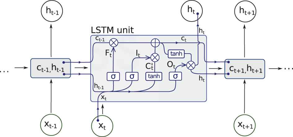
Long Short Time Memory (LSTM) cell structure.
Figure 2 shows a GRU cell. It is the new generation of recurrent neural network being very similar to LSTMs. A GRU structure does not have a state. So, the internal information is incorporated into its output. Thus, the number of parameters in the cell is reduced significantly. It also has only two gates, one for resetting (Equation (7)) and another one for updating (Equation (8)).
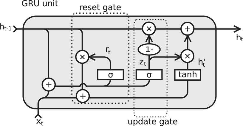
Gate recurrent unit (GRU) cell structure.
The input sequence tokens to RNN are taken one by one generating a fixed-sized vector. The way RNN work makes them ideal for several NLP tasks like machine translation [26–28] or speech recognition [29,30] among other. The way RNN work enhance their use for NLP. Some of its advantages are
The way to represent the networks input (a unit is modelled as a sequence) makes this network model the sequentiality of the language [4].
They can model texts with variable length. This ability leads them to deal with long sentences, paragraphs and documents [31].
RNN are able to summarize sentences, a useful quality in several NLP tasks such as automatic translation.
The network structure of RNN allows distributed processing, which benefits many NLP tasks such as multilabel text categorization [32], multimodal sentiment analysis [33] and subjectivity detection [34].
In spite of everything, it has not been shown that RNN outperform CNN. Yin et al. [35] conducted a comparative study of the performance of RNN and CNN in NLP tasks that their results are not conclusive; the performance of each network depends on the global semantics required by the task itself.
RNN lack of the ability to represent entries with natural recursive structure that occurs in natural language since words and subphrases are combined into phrases in a hierarchical manner. This problem is usually treated using structured tree models [36]. The recursive neural networks are appropriate since the representation of the nonterminal nodes in an analysis tree are determined by the representation of their children. These types of networks have been used successfully in NLP tasks such as parsing [37] or sentiment analysis [4].
RNN have been used at three levels in their application to NLP: (1) word classification; (2) sentence classification; (3) and language generation [4]. At the word classification level the use of bidirectional LSTM for NER have been proposed to capture context information of any length around the target word and generate two fixed-size vectors that were the input of another layer that performed the final labelling of the entity [38]. RNN represent an improvement to classical count statistics methods when they are applied to language modelling [4]. For example, Graves [39] presented the first work that proposed the use of deep RNN for language modelling. The use of a RNN to predict words was first proposed by Sundermeyer et al. [40]. They also suggested its applicability to a variety of different tasks, such as automatic statistical translation [41].
With respect to the sentence classification level, Wang et al. [42] proposed to encode complete tweets using LSTM. Their model allows to capture the effect of reversal of the word not. For the generation of responses it has also been proposed the use of Dual-LSTM [20] by selecting it from a set of candidate responses.
With regard to natural language generation it can be considered a typical RNN application. Deep LSTMs have been shown to generate reasonable text for automatic translation tasks, image captions, etc. In such cases, the RNN is called a decoder [4]. Sutskever et al. [28] experimented with 4-layer LSTM to perform automatic machine translation in an end-to-end fashion obtaining competitive results. This strategy has also been used to model human conversations [43]. Furthermore, extracting text from textual and visual clues is another research field in which these networks have been used [44,45].
We consider the proposal of Atteveldt [46,47] as the most similar one to ours. They presented a method to detect the subject and the predicate making use of the software Stanford CoreNLP [48] (a syntactic parser). This parser generates a particular parse tree and the authors oriented their proposal to the analysis of journalistic texts. They did not pretend to complete a syntactic analysis of the sentence; they tried to find out the subject and object of the action since its final aim was to show how corpus comparison and semantic network analysis applied to the results of the clause analysis can show differences in citation and framing patterns between U.S. and English-language Chinese coverage of this war [47]. The authors added a final phase called extracting clauses that found out the participants in the action from the tree parse generated by Stanford CoreNLP. Now, the architecture of the proposed model is shown.
3. MODEL ARCHITECTURE
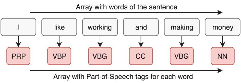
The model is composed by two neural networks. The first one is in charge of performing POS tagging. This network receives the words of the sentences and is trained to match each word with a POS tag (Figure 3).
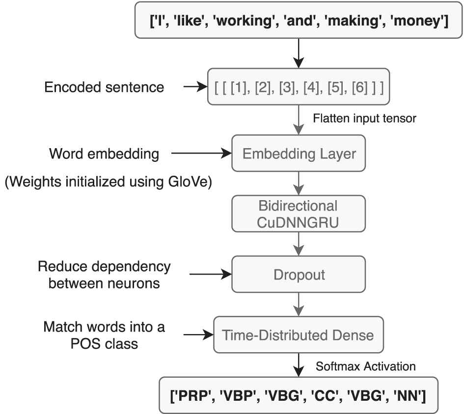
First network architecture.
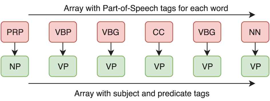
The second neural network receives POS tags as input, and it is trained to match each POS tag with a subject or predicate tag (Figure 4). Appendix details the set of tags we have used.
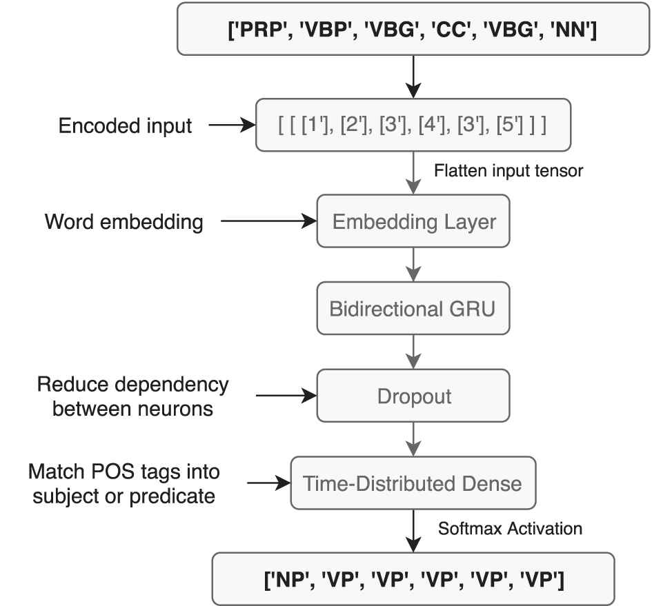
Second neural network architecture.
When making a new prediction, the words of the input sentence are provided to the first network, which makes a prediction obtaining a list of POS tags. Results obtained from the first network are provided to the second one, which matches each POS tag into subject or predicate class.
As described above, the first network matches the words with its POS tag, and the second network matches the POS tags into subject or predicate. By doing this, it’s intended to make it easier for the model to learn the rules for subject and predicate classification, since the number of POS tags is much more reduced than the word vocabulary. In Section 5, the results obtained with the model proposed in the paper versus a single network using the same architecture matching words into POS tags are compared.
Both networks use the same architecture: Recurrent neural networks based on gated recurrent units (GRUs) [49], which will be in charge of most of the learning process. When comparing with LSTM’s, GRU need less computational resources obtaining similar results.
The python code in Listing 1 is used to schematize the different layers in the model. It can be seen the structure of each layer and its configuration.
Listing 1 Scheme of the different layers in the model.
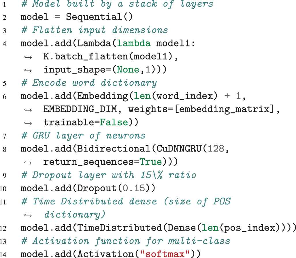
Defining the model as sequential means it’s built by a stack of layers (Line 2). The model is composed of the following layers:
Lambda Layer: It allows the model to work with different length sequences and it is necessary to flatten the input data. Using the batch_flatten function from the Keras library, a nD dimension tensor is reshaped to a 2D tensor. (Line 4).
Embedding Layer: This layer is intended to compress the word dictionary and also helps to find relationships between words. This layer aims to represent words using a dense vector representation with their relative meaning (Line 6). For the first neural network the model makes use of a pretrained word-vector representation model, the GloVe [50]. With this pretrained model, the weights of the embedding layer are initialized with those of the pretrained model. As an example, names like John and George would be related, so if the network learns that John is a name, by knowing the relationship between those words, it would predict George as a name too.
The second neural network does not use the pretrained word-vector representation model, since the input of this network are not words but the POS tags of the sentences that were used to train the first network.
Bidirectional GRU: The GRUs, usually known as GRU, were first proposed by Cho et al. [49] in 2014. As LSTM cells, GRU aim to solve the vanishing gradient problem. With these recurrent cells, it is able to remember information from past iterations. In this model, this type of network should be able to remember the information of past processed words and then use it in the next ones. The model uses GRU because they require less computational power than LSTMs, which leads to less training time. This layer uses 128 neurons on each direction (Line 8). With the bidirectional layer, the model processes the input sequences in forward and backward order, merging the knowledge from both directions at the output (Figure 5).
Dropout Layer: This layer is intended to prevent overfitting and dependency between neurons by shutting down 15% (0.15 ratio) of randomly chosen connections between neurons on each epoch for the first neural network, and 20% for the second one (Line 10). Dropout ratio is higher for the second network because the number of combinations of the input and output is significantly lower, since in the input there are only 53 possible POS tags, and in the output it only has the subject and predicate classes.
Time Distributed Dense Layer: This layer can be understood as an application of the different set of tags for each input token of the sequence, so it can be matched into one of the classes (Line 12).
Activation Function: The model uses the softmax activation function because of the nature of the problem: multi-class classification (Line 14).
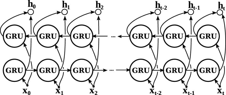
Scheme of the bidirectional gated recurrent unit (GRU) layer.
The incremental or online learning method (batch size of one sentence) that allows the model to process variable length input sequences for training was used. This method avoids the padding of the sequences and a memory waste with unnecessary tags which produces noise that is taken as input by the network. If this noise is not properly filtered it leads to an increment in the complexity of the model.
In contrast to batch learning, using incremental or online training implies some disadvantages:
More training is required for the same dataset, since the weights of the neurons are updated with each example. This could be a problem when using large datasets.
This type of training could lead to an unstable model. We have not experienced these problems in our model, but in order to prevent it we have decreased the standard learning rate set in the Keras library optimizers. Also we have added a dropout layer to prevent the possibility of overfitting problems.
The model uses the RMSprop optimizer which allows to obtain better results than the other optimizer used. We have also tested the Stochastic Gradient Descent (SGD) optimizer with Nesterov momentum and Adam optimizers, both configured with the same learning rate as the final one (lr=0,00001). When using SGD with Nesterov momentum set to 0.2, the model obtains about 30% less accuracy compared to RSMprop, probably because it requires a higher number of epochs. With the Adam optimizer, results were very similar than the obtained with RMSprop.
Other parameter to be defined in the model is the loss function. Since the problem has multiple categorical classes, the model is intended to use the sparse categorical cross entropy loss function instead of the categorical cross entropy. Using the categorical cross entropy loss function leads to the necessity of using one-hot encoding, which is not optimal when having a large number of classes.
4. DATASET
This section shows the preprocessing completed to adjust the dataset used as input of the network. The model uses the American National Corpus (ANC) [51], which is annotated following the Penn Treebank tagset. This notation can be easily interpreted by NLTK corpus readers when the dataset is imported. Then, we start importing the dataset using the Bracket Parse Corpus Reader [52] from NLTK library. All the sentences from the dataset are stored into a list. The imported sequence from the dataset has a tree structure (Figure 6). This tree usually splits into two main roots: subject (NP) and predicate (VP). The dataset has been revised and modified to be successfully applied to the model. In Figure 6 the format of a sequence directly imported from the dataset with the corpus reader is shown.
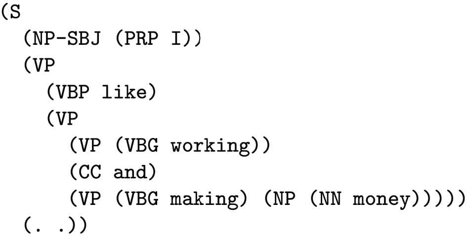
Imported sequence from American National Corpus (ANC) Corpus.
A recursive function is used to iterate over each sentence and build two lists: One that contains the words of the sentences, and in other one to store the tags for each word. The input sequences from the dataset to the function are NLTK Tree objects. The function start iterating over each node of the tree, storing the tags of each node. When reaching a word (the leaf of the tree), the tags explored by the function until reaching the leaf are stored in the list of tags, and the leaf is added to the list of words.
The generated lists contain errors and to accomplish these the following modifications are done over the lists:
Delete sequences with less than two words. Most of them contain unusable characters.
Split tags separated by ”=,” reducing the number of classes to be used by the model. The extra information contained in these tags is not required for this problem, in fact, it is better to reduce the number of classes. This can be observed in the following example:
[’S’, ’S’, ’VP=2’, ’PP’, ’NP’, ’:’]
is replaced by
[’S’, ’S’, ’VP’, ’PP’, ’NP’, ’:’]
Delete empty elements that cause errors in the network. This elements were introduced by faulty tokens when importing the dataset. This can be observed in the following example:
[’S’, ’NP’, ”]
Split sentences which contain “.”, “,”, “:“, “/”. By doing this, the total number sentences increases, decreasing the length of some sentences that were excessively long (more than 50 words). This can be observed in the following example:
[…, ’to’, ’Goodwill’, ’in’, ’1998’, ’,’, ’we’, ’helped’, ’our’, …]
is replaced by the following lists:
[…, ’to’, ’Goodwill’, ’in’, ’1998’] and [’we’, ’helped’, ’our’, …].
Delete words which start with ’*’ or ’-’. These elements are used to mark unidentified words. Deleting these elements allows to prevent the network from learning nonexistent words. This can be seen in the following example:
[’if’, ’we’, ”’re”, ’not’, ’called’, ’*-1’, ’today’]
is replaced by:
[’if’, ’we’, ”’re”, ’not’, ’called’, ’today’]
Make sure every list of tags for each word starts with the “S” tag, to check every list of tags is following the same formatting style.
After the preprocessing, two lists are obtained:
sentences: Contains the words of the sentences. This variable matches with the first column of Figure 7.
tags: Contains a list for each word with all the tags found over the three. This variable matches with the rest of the columns of Figure 7.
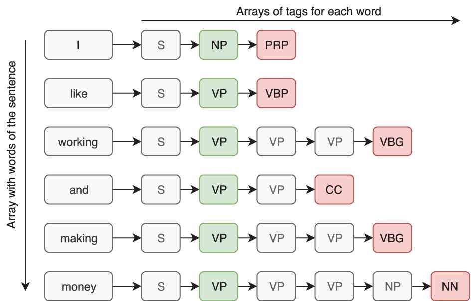
Data relationship between the two variables.
Then, the input lists are built for the first and second neural network in the following way:
The input for this network are the words of the sentence. This data is exactly the same than the sentences variable, so nothing else is required to obtain it (first column in Figure 7).
[’I’, ’like’, ’working’, ’and’, ’making’, ’money’]
For training, this network uses the POS tags of the words. To get this data, we build a new variable containing for each word of a sentence, its POS tag (Appendix). For each word, this tag is located at the final position of the tags array. To extract these POS tags it is needed to use the second built variable. It is highlighted in red in Figure 7, i.e., [’PRP’, ’VBP’, ’VBG’, ’CC’, ’VBG’, ’NN’] (Figure 8).
The second network receives as input the POS tags of each word (Figure 8):
[’PRP’, ’VBP’, ’VBG’, ’CC’, ’VBG’, ’NN’]
The target data for this network is the subject and predicate tags for each word. To build this data, a new variable is created containing the subject or predicate tag for each word. To extract this information the tags variable obtained after the preprocessing is used, saving into the new variable the first detected NP of VP tag of the array for each word. This information is highlighted in green in Figure 7 (Figure 9).
[’NP’, ’VP’, ’VP’, ’VP’, ’VP’, ’VP’]
First NN data.
Second NN data.
Not every list of tags contains subject or predicate tag for each word. For example, connectors are not classified neither as subject or predicate. Only the words which contain subject or predicate are used, both for the first and the second networks, so related sets are used. Finally, there are a total number of 8775 samples prepared to be used within the model. Before they are passed to the network, the lists are encoded to numbers using the Keras Tokenizer. Then, the arrays are converted to numpy arrays, and the dimensions are modified so they can be processed by the network for the online/incremental training process. As an example, this sentence with shape (6, ): [’1’, ’2’, ’3’, ’4’, ’5’, ’6’] is reshaped to (1, 6, 1): [[[’1’], [’2’], [’3’], [’4’], [’5’], [’6’]]].
5. RESULTS
This section talks about how the training process is completed, the tools used to make the tests and the results obtained. The results obtained with the model will be compared with other similar tools. The first neural network has been specifically compared with the tool to assign tags provided by NLTK (NLTK.pos}_tag()), and the second one has been compared with an statistical tool named pyStatParser. In these tests the ANC[51] has been used. This corpus can be obtained in the following url: http://www.anc.org/MASC/download/penn-treebank.zip (Last visited on 17 Nov. 2019). This dataset has been preprocessed following the procedure detailed in Section 4 obtaining a total number of 8775 samples ready to be used in the tests. From this set, a 70% has been used for training and a 30% for testing the networks, i.e., the model has used 6142 samples for training and 2633 for testing. Before splitting the dataset into training and testing it is randomly merged. To do this, the train_test_split function from the scikit learn library, with the shuffle parameter marked as True has been used.
The proposed model has been implemented using the Python 3 programming language. Tensorflow [53] 1.15.0 and the Keras API included in this Tensorflow release (2.2.4-tf) have been the main libraries used in the development of the model. The main reason to use these libraries is that they provide the tools to implement the developed model. Furthermore, because of their popularity lots of different kind of resources about them can be found on media. Google Colaboratory [54] has been used as the main development environment, making use of a free GPU instance, which provides an NVidia Tesla K80 GPU. NVidia GPU’s are popular in Machine Learning field because of the compatible libraries from NVidia as the CuDNN library. This library includes optimized GRU cells to be efficiently executed on compatible NVidia hardware. That is the reason why the model makes use of CuDNNGRU. If someone wants to replicate the experiments write to the contact author.
The following sections detail the tests done for the first and second neural networks (Sections 5.1 and 5.2) and the comparative tests (Section 5.3).
5.1. Testing the First Neural Network
The first network was trained with 25 epochs, so the network has used this training set in total 25 times. While training, accuracy and loss variables were recorded. These are obtained for every sentence but is more relevant to measure them for each epoch. So, to obtain the values for each epoch, the arithmetic mean over the recorded values for each sentence during each epoch is used. Once finished the training process, the logs can be represented using graphs as it can be seen in Figures 10 and 11.
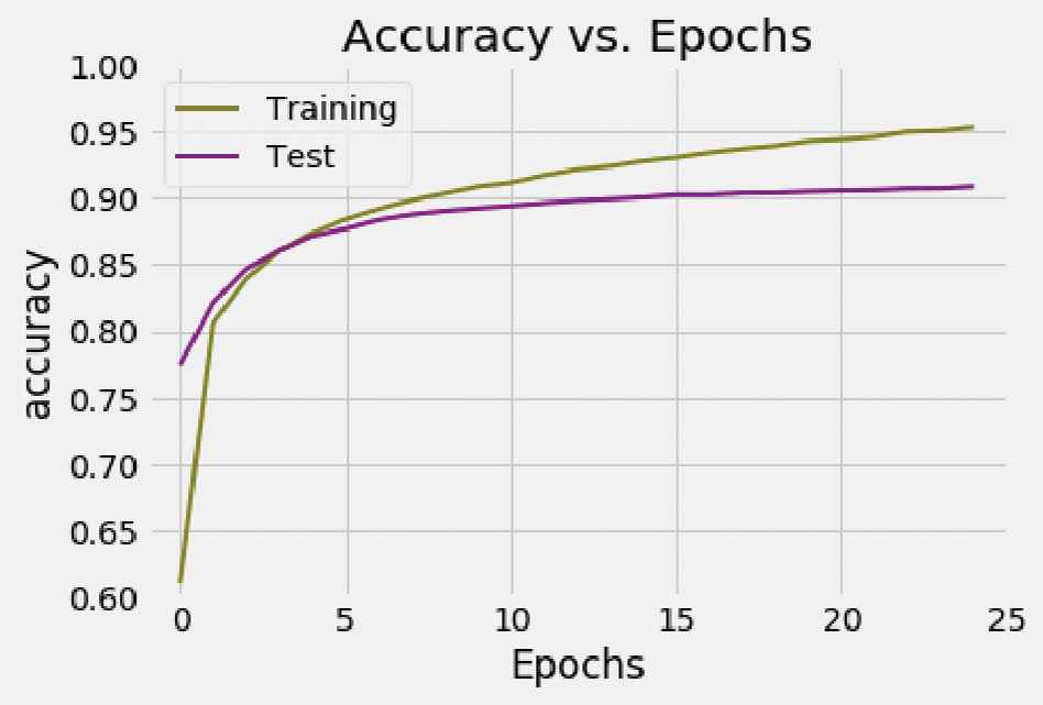
Accuracy vs. Epochs—first network.
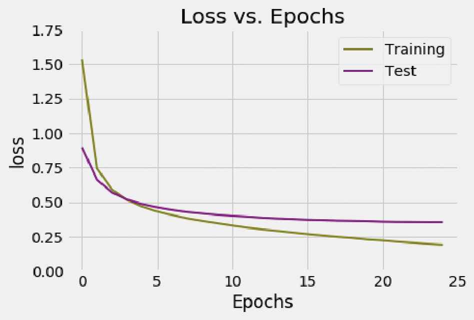
Loss vs. Epochs—first network.
Figure 10 shows the evolution of the accuracy on each epoch while training the first network. It quickly increases at the beginning of the training process, and then progressively gets stabilized until no insignificant improvement in accuracy is gotten. The training process was repeated a different number of epochs, trying to find an equilibrium between training time and results obtained, and also avoiding overfitting. The optimal number of epochs was found to be 25. The accuracy obtained for the training set is 95.12%. When benchmarking with the test set, it is obtained an accuracy of 90.38%, lower than the one obtained with the training set. We believe these scores are acceptable because they surpass the 90% in both cases. The loss obtained for the training set is 0.1960 and 0.3563 for the test set. Figure 11 details the loss evolution for the 25 epochs. As it has been seen with respect to the accuracy, it get stabilized around the considered optimal of 25 epochs. These values could be considered acceptable since both are less than
5.2. Testing the Second Neural Network
The second network has been trained with a total number of 20 epochs, using the same method than previously to record the accuracy and loss logs for each individual epoch. The logs can be seen in Figures 12 and 13.
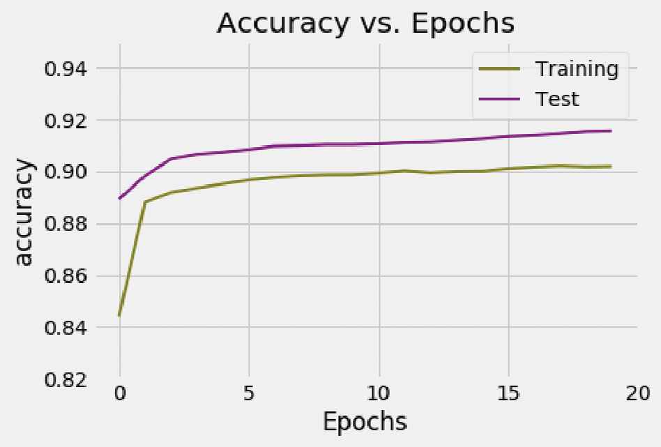
Accuracy vs. Epochs—second network.
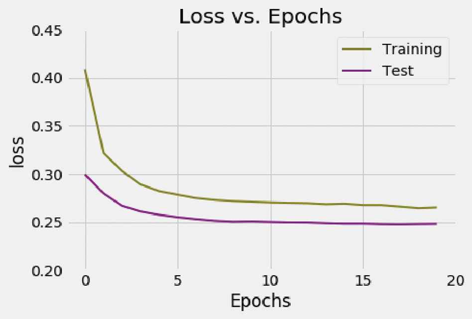
Loss vs. EpochsSecond network.
The accuracy obtained for the training set is 90.17% and 91.55% for the test set. It is noteworthy that the accuracy value obtained using the same set of examples used for training obtains results very similar to those obtained when the set of tests is used. The loss value is 0.2652 for the training set and 0.2480 for the test one. Again, these values could be considered acceptable since both are less than 0.5.
In the obtained graphs (Figures 10–13) it can be observed that during some concrete epochs with respect to the first NN, and for every epoch in the second NN, the accuracy values obtained for the test set are higher than the obtained for the training set. This behavior is the opposite of what could be expected and it comes motivated by the dropout layer, that shuts down some of the connections between neurons (randomly selected in each epoch) to prevent overfitting and dependency between neurons. The values obtained for the training set occurs with these neurons off, while on the test set the model uses the whole computational power being this the reason why these results are obtained.
5.3. Comparative Results
The model proposed in this paper has been compared against different tools that aim to perform the same task. Due to the fact that our model is composed of two networks, we have compared the results for each network individually.
The first neural network of our model matches the words of an input sentence with their POS tags. We have compared this network with the tool from NLTK library NLTK.pos_tag() and also against spaCy, an open-source library for NLP [55].
In relation with the second neural network, it has not been found any tool similar to the second network which matches POS tags into subject and predicate. The model has been compared against pyStatParser [12], a statistical parser tool which performs complete syntactic analysis to an input sentence, comparing the subject and predicate tags predicted by this tools with the ones obtained by our second network. From the results obtained (Table 1) it can be verified that both methods obtain practically the same results, so we can affirm that results of our network are comparable to the ones obtained by the NLTK.pos_tag (), a tool frequently used in this class of tasks. spaCy presents a slightly lower performance than our approach.
| Tool | Accuracy (%) |
|---|---|
| Neural network 1 | 90.3876 |
| NLTK pos_tag() | 90.1560 |
| spaCy | 88.9684 |
Comparison of the first neural network.
The model accuracy in subject and predicate classification has been also compared against a single network that matches words of a sentence straightforward into subject or predicate. This network is based on the same architecture as those used with the dual network model proposed in the paper. Therefore it’s based on a Bidirectional GRU layer using 128 cells. Thus, the main difference between this network and those used for the dual model is the data it uses. This network receives the words of a sentence and at the output it’s obtained a subject or predicate tag per each word. From the results obtained (Table 2), it can be seen how the model proposed in the paper slightly improves the scores obtained with one network.
| Tool | Accuracy (%) |
|---|---|
| Neural network 2 | 0.8767 |
| Single network | 0.8664 |
Comparison of second NN vs. single network.
As it can be observed in Table 3, the performance obtained by our network is far superior than the one obtained by pyStatParser, although it must be remarked that the performance of pyStatParser can be considered poor. Furthermore, pyStatParser failed when analyzing some sentences, so those that generated errors were excluded from the testing set for this comparison.
| Tool | Accuracy (%)a |
|---|---|
| Neural network 2 | 91.7432 |
| pyStatParser | 61.5887 |
Score obtained excluding from test set the sentences which caused errors with pyStatParser.
Comparison of second NN vs. pyStatParser.
The technique presented in this paper can be used in the field of document classification. At present, a large number of documents are generated and they must be classified. Machine learning techniques are often used to solve it [56].
6. CONCLUSIONS AND FUTURE WORKS
In this paper it has been presented a neuronal network model that makes the syntactic analysis of a sentence determining its subject and its predicate. The model consists of two recurrent neural networks based on GRU. A sentence is the input of the first network and its output is taken as input for the second network. The first network makes the POS tagging of each sentence, while the second one indicates for each word whether it is a component of the subject or of the predicate. To prepare the input of our model, the preprocessing of a syntactic tree generated by NLTK in Penn Treebank tagset format has been done, obtaining the input structures to our model. As dataset, the one provided by “The Open ANC” has been used. The model training has used a 70% of the samples while the remaining 30% have been used for the tests. For the comparison, in our review we have not found any tool in the literature that can be compared in a direct way to the model proposed. For this reason, we have compared with the labelling tool provided by NLTK for the first neural network, and with a parser called pyStatParser for the second neural network. The results obtained by the first neural network are similar to those obtained by the labelling tool provided by NLTK. The second neural network has far exceeded pyStatParser, although the performance of this parser can be considered as weak. To sum up, it can be said that the results obtained are acceptable since both networks exceed the results obtained by the method with which it has been compared. In addition, the accuracy of the two networks that make up the model exceeds 90% and the loss is less than
We will seek the development of improved models based on the work exposed in this paper. We pursuit the development of a more complex network which would be able to perform complete syntactic analysis of sentences. Even though we focus our major efforts on RNN, we don’t discard testing other network architectures, such as CNN. All this research is aimed at achieving the classification of documents in Section 5.
ACKNOWLEDGMENTS
This work was funded by the project TIN2015-64776-C3-3-R of the Science and Innovation Ministry of Spain, co-funded by the European Regional Development Fund (ERDF), and by the Information Systems and Technologies Department of the University of Castilla-la Mancha.
APPENDIX
| Index | Tag | Meaning |
|---|---|---|
| 0 | -PAD- | Padding |
| 1 | CC | Coordinating conjunction |
| 2 | CD | Cardinal numbers |
| 3 | DT | Determiner |
| 5 | FW | Foreign word |
| 6 | IN | Proposition or subordinate conjunction |
| 7 | JJ | Adjective |
| 8 | JJR | Comparative adjective |
| 9 | JJS | Superlative adjective |
| 11 | MD | Modal |
| 12 | NN | Noun singular |
| 13 | NNS | Noun plural |
| 14 | NNP | Proper noun singular |
| 15 | NNPS | Proper noun plural |
| 16 | PDT | Pre-determiner |
| 17 | POS | Possessive ending |
| 18 | PRP | Personal pronoun |
| 19 | PRP$ | Possessive pronoun |
| 20 | RB | Adverb |
| 21 | RBR | Adverb, comparative |
| 22 | RBS | Adverb, superlative |
| 24 | SYM | Symbol |
| 25 | TO | “to” |
| 26 | UH | Interjection |
| 27 | VB | Verb, base form |
| 28 | VBD | Verb, past form |
| 29 | VBG | Verb, gerund or present participle |
| 30 | VBN | Verb, pasta participle |
| 31 | VBP | Verb, non-3rd person singular present |
| 32 | VBZ | Verb, 3rd person singular present |
| 33 | WDT | Wh-determiner |
| 34 | WP | Wh-pronoun |
| 35 | WP$ | Possessive wh-pronoun |
| 36 | WRB | Wh-adverb |
| 37 | S | Sentence |
| 38 | NP | Noun phrase |
| 39 | VP | Verb phrase |
Table A.1 Tagset meaning.
REFERENCES
Cite this article
TY  - JOUR
AU  - David Muñoz-Valero
AU  - Luis Rodriguez-Benitez
AU  - Luis Jimenez-Linares
AU  - Juan Moreno-Garcia
PY  - 2020
DA  - 2020/06/17
TI  - Using Recurrent Neural Networks for Part-of-Speech Tagging and Subject and Predicate Classification in a Sentence
JO  - International Journal of Computational Intelligence Systems
SP  - 706
EP  - 716
VL  - 13
IS  - 1
SN  - 1875-6883
UR  - https://doi.org/10.2991/ijcis.d.200527.005
DO  - 10.2991/ijcis.d.200527.005
ID  - Muñoz-Valero2020
ER  -