1. INTRODUCTION AND BACKGROUND

Sepsis is a syndrome of severe systemic reaction caused by infection. It is a common complication of various traumas, burns, shock, injuries and large-scale surgical operations. The deterioration in the condition of sepsis patient develops rapidly. Despite the advancement in diagnosis and treatment technologies and monitoring measures, the morbidity and mortality of sepsis are still relatively high, which is a global challenge facing the health systems. According to severity, sepsis can be divided into three levels, which are sepsis, severe sepsis and septic shock. In addition to inflammatory symptoms, severe sepsis and septic shock patients also have organ dysfunction, hypotension or poor tissue perfusion, which can endanger the patient's life in serious cases. Studies have shown that patients with critical sepsis also exhibit persistent arterial hypotension after fluid resuscitation, which may be one of the important factors affecting the development of the disease [1]. As a result, it is important to control blood pressure when the patient is in the case of hypotension.

Today, artificial intelligence (AI) technologies are being widely employed in medical research and practice. A number of research has focused on medical time series data for diagnosis or assistance in early detection. C. Barajas, R. Akella regarded the probability of mortality as a time-based state and estimated it inside the intensive care unit (ICU) according to medical time series data [2]. I. Batal et al. proposed the STF-Mine algorithm to abstract temporal features from patients' time series data, and classified the data based on these features [3]. A. Taoum et al. used the time series data of four basic vital signs to construct an early warning model of acute respiratory distress syndrome (ARDS) using machine learning and statistical knowledge [4,5].

Long short-term memory (LSTM) network is a commonly used method for time series data analysis because of its advantage in processing and predicting sequence data. Z. C. Lipton et al. used LSTM network to diagnose the main kinds of diseases from multivariate time series of clinical measurements [6]. B. K. Beaulieu-Jones et al. proposed a type of LSTM network to predict the survival status of patients one year after admission based on the time series data recorded during patient care in MIMIC-III [7]. H. G. Kim et al. used LSTM network to predict medical examination results according to medical examination data from previous years [8]. The result can give the patients a chance to early detect the disease. The time interval of medical time series data is usually irregular, which may affect the predict results of LSTM. To solve this problem, I. M. Baytas et al. proposed a new LSTM unit [9]. Although these technical approaches are widely used for medical time series analysis, to the best of our knowledge, there is presently no published work that uses LSTM networks to adjust the dose of medication and regulate blood pressure. Distinguished from existing works using LSTM in the medical field mentioned above, adjusting the patient's blood pressure requires considering the patient's multiple vital signs historical data, and making high-frequency, real-time prediction especially in short time.

In recent years, there also exist related studies combining AI technology with the treatment of sepsis. However, studies on the dose adjustment of vasopressors in sepsis patients are few in numbers. In Refs. [10–12], the treatment process of sepsis was regarded as a sequential decision-making problem. They found that most of the treatment decisions made by human clinicians are suboptimal for patients, so they developed AI clinicians who can learn optimal treatment through reinforcement learning. However, the purpose of these works is to reduce the mortality in patients and the dose for vasopressors is discretized into five bins, which cannot predict the precise dose of vasopressors at the next state. Moreover, one property of Markov model-based decision-making process is memoryless, and the dose at the next moment can only be predicted based on the current state, which is different from LSTM that can utilize current and historical state data for prediction.

In this paper, we propose an LSTM network approach to predict the dose of norepinephrine, a kind of vasopressors recommended by guidelines, based on medical time series data of sepsis patients collected in the MIMIC-III database. The purpose of our work is to validate whether may design a learning-based model to simulate doctor's behavior for dose regulation effectively in order to help doctors to control the patient's blood pressure in time. We attempt to cluster the patient clinical data according to the changes of historical dose, vital signs and laboratory test results, and explore whether it can be helpful to improve the effect of dose regulation. This may provide the enlightenment for doctors to further lean treatment through the analysis of the correlation between different dimensions and the difference between the prediction results before and after clustering. Due to the limit on the number of doctors and caregivers, compared to the number of patients suffering from the condition, this research has the real signification on reducing the burden on doctors and caregivers.

2. METHOD

2.1. Data Preprocessing

2.1.1. Data resource

MIMIC-III is a large, freely-available, single-center database comprising information relating to more than 40,000 patients admitted to critical care units of the Beth Israel Deaconess Medical Center between 2001 and 2012. The database includes information such as demographics, vital sign measurements made at the bedside (one data point per hour), laboratory test results, medications, caregiver notes, diagnostic codes, imaging reports, hospital length of stay and survival data, etc. It supports a diverse range of analytic studies spanning epidemiology, clinical decision-rule improvement and electronic tool development [13].

We obtained approval to use the database (Certification Number: 27959316) for our research, after completing the National Institutes of Health (NIH) web-based training course: Protecting Human Research Participants.

2.1.2. Collection of samples

In our experiment, we focus on the information of those sepsis patients who meet the following criteria:

1. Sepsis-related organ failure assessment (SOFA) is not less than two points.

2. Use only norepinephrine to regulate blood pressure, without using other blood pressure regulating drugs such as dopamine, adrenaline and vasopressin.

3. Not younger than 18.

4. Nonsurgical ICU-hospitalized patients.

5. In order to observe and analyze time-series data, the dose of norepinephrine has to be adjusted at least five times continuously according to the changes in vital signs and laboratory test results.

Here Criteria (i) is the international diagnostic criteria of sepsis patients. Norepinephrine is recommended in the international guidelines as the first choice of vasopressor for the treatment of hypotension caused by sepsis [14]. Of all patients who met the sepsis criteria and used vasopressor, 72.47% used norepinephrine first. Meanwhile, children of different ages have different response intensity to vasoactive drugs, and the guideline only give advice for adults to use norepinephrine, so we excluded patients younger than 18. The reason why we only focused on the nonsurgical ICU-hospitalized patients is that the development process of sepsis caused by surgery and trauma is different from general sepsis.

Based on the above criteria, we obtained clinical data of 541 patients from MIMIC-III. Then, their data about the adjustment of the dose of norepinephrine is collected, including the start time and the end time of the adjustment, and the dose of norepinephrine at this time period. We also collect age, gender, Glasgow Coma Scale (mingcs), key vital signs and patient's laboratory test results including Bilirubin, PaO2, FiO2, Creatinine, WBC, mean arterial pressure (MAP), Respiratory Rate, Heart Rate, Temperature in C, SPO2 and PEEP at every intervention point. Because the normal value range of the dose is 0-0.2 mcg/(kg⋅min), so we regard the data in which the dose is above 2 mcg/(kg⋅min) as the outlier and delete them.

2.1.3. Preprocessing and extraction of time series data

In the collected samples, there exists noisy data and missing values. Therefore, we need to consider how to fill in the missing values. First, we count the missing rate for each variable. Figure 1(a) shows the result. For each patient, we fill in the missing values of each variable by the average of this patient's data. Then, we count the missing rate of each variable again and the result is shown in Figure 1(b). There still were reasonable amounts of missing values. For these missing values, we fill them by the average of all the patients' data. But as the missing rate of FiO2 is up to 45.4% before the first filling and 37.9% after the first filling, we delete this variable.

Figure 1

The missing rate of each variable before and after the first filling.

After filling the missing values, the value range of all the variables of vital signs and laboratory test results are converted into [0,1] by the way of min-max normalization. Then, we construct multidimensional time series data X=X1,X2,…,XL with the patient's data we collected. Each time step Xi is a 14-dimensional vector, including the dose at previous time step (if there is no previous time step, the value is zero), age, gender, mingcs, Bilirubin, PaO2, Creatinine, WBC, MAP, Respiratory Rate, Heart Rate, Temperature in C, SPO2 and PEEP. The data is processed into time series data of the same length. Figure 2 shows the process to generate time series that the length L equals to seven.

Figure 2

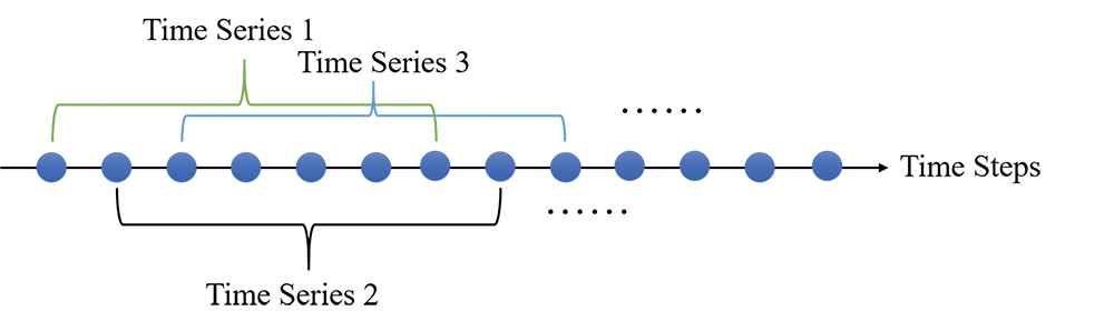
The process to generate time series that the length L equals to seven.

2.2. Prediction Model Based on LSTM

In this subsection, we present a prediction model based on the LSTM network technique to predict the dose of norepinephrine at the last time step. LSTM network is an improvement of recurrent neural network (RNN), which is mainly used to process and predict the sequence data, and can solve the problem of gradient disappearance and gradient explosion caused by back propagation and long-term dependence, as it performs better than RNN in various areas, such as speech recognition [15,16] and natural language processing [17,18]. Figure 3 shows the structure of one cell and its evolution through time [19].

Figure 3

Structure of a long short-term memory (LSTM) cell and its evolution through time. The thick arrows indicate the evolution through time.

Eqs. (1) to (6) give the update for cell state ct and final output ht at time step t, where σ and tanh stand for the element-wise application of the sigmoid (logistic) function and tanh function respectively, and ⊙ is the Hadamard (element-wise) product. xt is the input at time step t, W and U are parameter matrix and b is the bias.

ft=σ(Wfxt+Ufht−1+bf)(1)

it=σ(Wixt+Uiht−1+bi)(2)

ot=σ(Woxt+Uoht−1+bo)(3)

c˜t=tanh(Wc˜xt+Uc˜ht−1+bc˜)(4)

ct=ft⊙ct−1+it⊙c˜t(5)

ht=ot⊙tanh(ct)(6)

Dropout is a mechanism often used in deep neural networks to make the network more robust and prevent overfitting by stopping the work of a certain cell with the probability p in the process of forward propagation of the network. In the deep RNN, which has more than one recurrent layer, dropout is only used between cells in different recurrent layers at the same time step.

In this work, we design an LSTM network with two recurrent layers with the dropout mechanism used between them. Figure 4 shows the structure of the whole network used in our work. This LSTM network receives a medical time series data X=X1,X2,…,XL as input, and the input at the l-th time step Xl is a 14-dimensional vector mentioned above, including the dose at the previous time step, vital signs and laboratory test results. L is the length of the time series. Then, the prediction of the dose at the last time step ŷ is the output of the whole network. Because the output of the two-layer LSTM network at the last time step is a multidimensional vector rather than a numerous value, we add a fully connected layer to make the final output as a numerous value. Mean absolute error (MAE) is used as the cost function of the whole dataset with M time series data:

MAE=1M∑i=1Mŷi−yi(7)

where ŷi and yi are respectively the prediction value and the true value of the dose at the L-th time step of the i-th time series data.

Figure 4

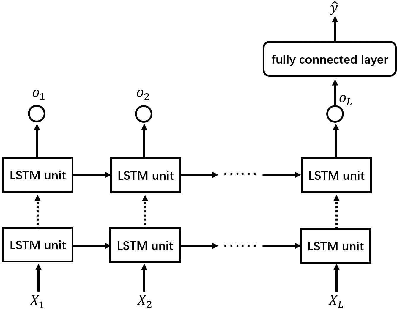
The structure of the network used in this work. The dotted arrows between two recurrent layers represent the use of the dropout mechanism.

2.3. Measurement of the Similarity of Time Series and Clustering Analysis

We use K-means algorithm to cluster time series data in our work. Measuring the similarity between samples is a very important step in the process of clustering data. Therefore, we need to measure the similarity of time series when we cluster the data. Another important step of K-means algorithm is to specify the number of clusters K. However, we often do not know how many clusters of raw data are most suitable. Therefore, we need to use some methods to help us determine the number of clusters correctly. At present, some scholars have proposed several advanced K-means algorithms that can automatically determine the most suitable number of clusters [20–22]. In our work, we choose the parameter K via silhouette coefficient. This subsection describes two common methods to measure the similarity of time series and the concept of silhouette coefficient.

2.3.1. Euclidean distance

Euclidean distance is a commonly used method to measure the distance between two points in n-dimensional space when we use K-means algorithm to cluster data [23–25]. For two points in n-dimensional space, P=(p1,…,pn) and Q=(q1,…,qn), the Euclidean distance D between them is defined as Eq. (8).

D(P,Q)=∑i=1npi−qi2(8)

For m-dimensional time series data of length n, we can regard it as a point in the n×m dimensional space. In this way, we can use the Euclidean distance to compare the similarity of time series: the closer the distance, the higher the similarity; the farther the distance, the lower the similarity. However, Euclidean distance is only suitable for comparing time series with equal length. Moreover, since we regard time series data as a point in the n×m dimensional space, we ignore the trend of time series over time.

2.3.2. Dynamic time warping

The dynamic time warping (DTW) algorithm is an efficient way to measure the similarity of time series because through temporary changes in the time series for discerning similar objects and shapes for its different phases has allowed for the minimizing of effects caused by shifts and distortions [26]. There are also a series of work, which used DTW as the similarity measurements in clustering analysis [25,27,28]. Compared with the Euclidean distance, DTW algorithm can measure the similarity of two time series with different length. Figure 5 shows the different ways in data alignment between Euclidean distance and DTW.

Figure 5

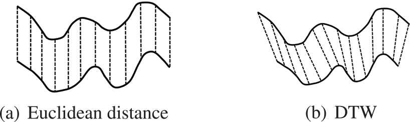
Different ways in data alignment between Euclidean distance and dynamic time warping (DTW).

The dynamic programming idea can be used when programming the DTW algorithm. Suppose there are two time series P=p1,p2,…,pn and Q=q1,q2,…,qm with the length of n and m respectively, DTW(P,Q) can be calculated by recursive formula Eq. (9), where 1⩽i⩽n,1⩽j⩽m. d(pi,qj) represents the square of the Euclidean distance of the data point pi at the i-th time step in P and the data point qj at the j-th time step in Q, so d(pi,qj)=(pi−qj)2.

S1,1=d(p1,q1)S0,j=Si,0=+∞Si,j=d(pi,qj)+min{Si−1,j,Si,j−1,Si−1,j−1}DTW(P,Q)=Sn,m(9)

2.3.3. Silhouette coefficient

Silhouette coefficient is a measure of how similar a data point is to its cluster compared to other clusters [29]. Assume the data has been clustered into K clusters by K-means algorithm. For the data point x, which is in the cluster Ci, calculate the average distance ax between the data point x and all other data points in the clusters Ci:

ax=1Ci−1∑y∈Ci,x≠yd(x,y)(10)

where d(x,y) is the distance between data point x and y. Then calculate the average distance between the data point x and all the data points in any other cluster and choose the minimal one as bx:

bx=mini≠j1Cj∑y∈Cjd(x,y)(11)

Now we can define the silhouette coefficient of date point x as

sx=bx−axmax(ax,bx)(12)

The average of all the silhouette coefficient of each data point s is defined as the silhouette coefficient of the whole dataset. From the definition above, we know that the value of s is in the range of [−1,1]. The larger the s, the more the results of clustering can reflect the true distribution of data. So, we choose the value of K that makes the s the biggest.

2.4. Experiment Setting

Before the experiment started, we needed to choose a proper length of the time series. First, the medical sequence data we collected is divided into sub-sequences with the same length L, and the value range of L is 5 to 15. Figure 6 shows the number of sub-sequences when L changes. Then we predict the dose of norepinephrine ŷ at the last time step based on the dose, vital signs and laboratory test results at the past time steps with a simple LSTM network with only one hidden layer and calculate MAE by comparing to the actual dose y on each dataset. Five-fold cross validation is implemented in our experiment. We can get the lowest MAE when L equals to ten, so the proper length of time series should be ten. Eventually, 314 patients remained whereas the times of the adjustment of other patients are less than ten.

Figure 6

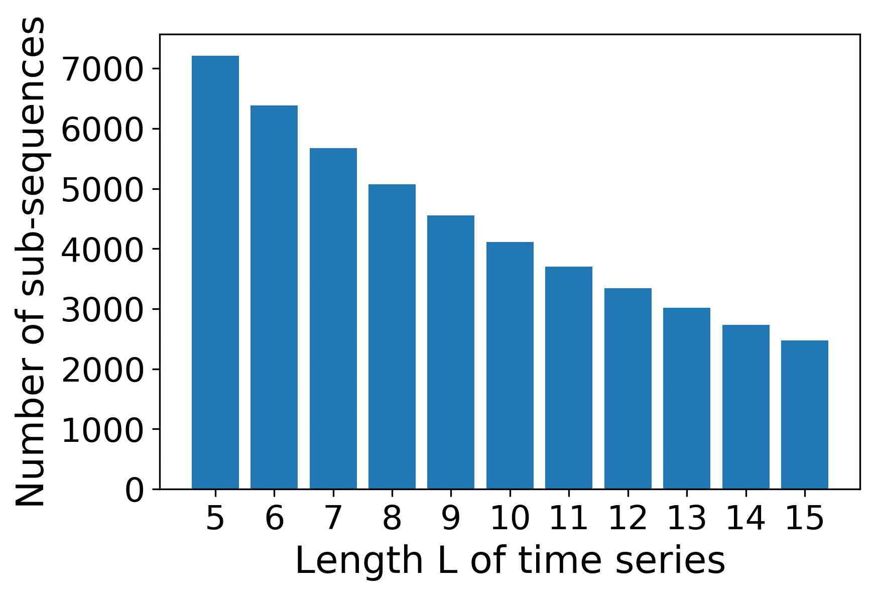
The number of sub-sequences with different L.

After choosing the proper length of the time series, we use the model proposed here to predict the dose of norepinephrine on the chosen dataset and calculate the MAE by five-fold cross validation. Then, we construct two regression models to compare with the model we proposed. Two regression models, linear regression and XGBoost regression [30], both predict the dose of norepinephrine based on the dose at previous time step and the value of vital signs and laboratory test results at the current time step. Linear regression is a simple regression model. It learns the regression equation and determine the regression coefficients from the training data. Then, the prediction result is obtained by calculating the regression coefficient and the input. XGBoost, namely Extreme Gradient Boosting, is an ensemble learning method based on classification and regression tree (CART) as basic learner. XGBoost performs a second-order Taylor expansion on the cost function when optimizing the cost function to improve efficiency. It also effectively controls the complexity of the model by adding regularization. XGBoost usually has a better learning effect than traditional machine learning algorithms.

Then, the K-means algorithm, based on two different time series similarity measures, i.e., Euclidean distance and DTW, is used to cluster the data according to the changing trend in patient historical data. The purpose of clustering is to explore whether clustering analysis can be helpful to improve accuracy and effects on dose adjusting. We do not consider two discrete variables, gender and mingcs, while clustering because it is meaningless to consider the changing trend of these two variables since the values of a patient do not change during the monitoring process. So, the data being clustered is 12-dimensional time series of length ten. The number of clusters is determined by silhouette coefficient. According to the number of clusters, the same number of LSTM network models shown in Figure 4 are constructed. On each cluster, we train the respective model with the 14-dimensional data and get the MAE on this cluster using five-fold cross validation. The total MAE on the whole dataset will be calculated as Eq. (13), where K is the number of clusters, MAEi is the MAE on cluster i, Mi is the number of time series on cluster i and M is the number of time series of the whole dataset.

MAEtotal=1M∑i=1KMAEi×Mi(13)

3. RESULTS

3.1. Variables Analysis

Among all the variables we chose, gender and mingcs are discrete variables, and others are continuous variables. For all the continuous variables, we count their data distribution, and then draw their data distribution histograms and probability density functions, as shown in Figure 7. We can see that all the continuous variables are basically in accordance with the normal distribution except for PEEP. There are also some outliers in the data. For example, 99.1% of the data in WBC is less than 40K/uL but the max value is 471.7K/uL.

Figure 7

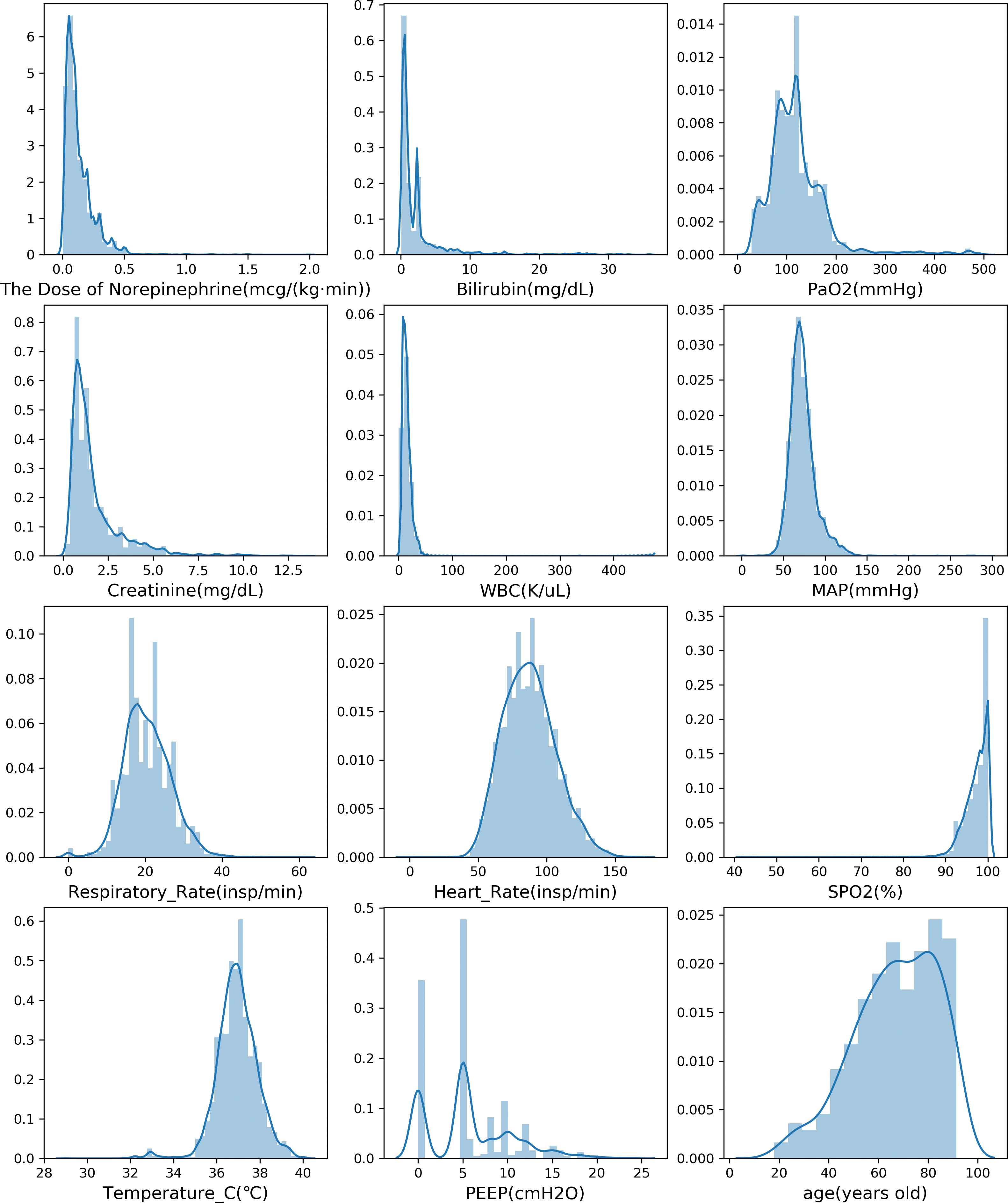
The data distribution histograms and probability density functions of continuous variables.

Then, we calculated the absolute value of Pearson correlation coefficient between pairs of variables that basically fit a normal distribution, as shown in Figure 8. We can see that the absolute values of all coefficients are closer to 0 compared to 1, indicating that there are no two variables with strong linear correlation.

Figure 8

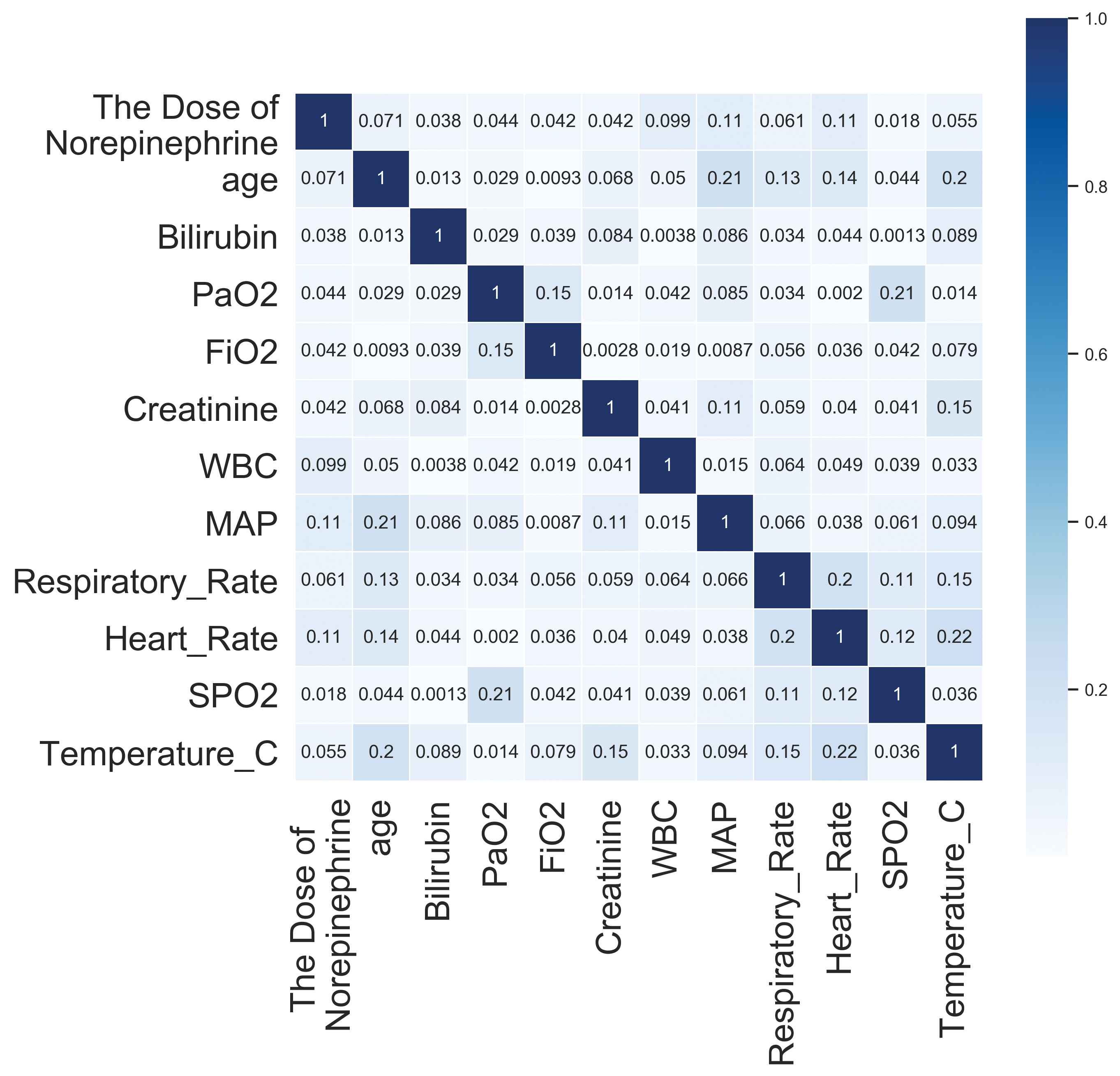
The absolute value of Pearson correlation coefficient between pairs of variables that basically fit a normal distribution.

For the discrete variables, gender and mingcs, the data distribution is also counted, and the data distribution histograms are shown in Figure 9. Since mingcs is always the same for one patient during the monitoring process, multiple repeat of mingcs data for one patient are counted only once. We use the same method to count the data distribution of gender and age. Figure 9. shows that there are slightly more male patients than female patients, and more than half of the patients are always in a state of consciousness.

Figure 9

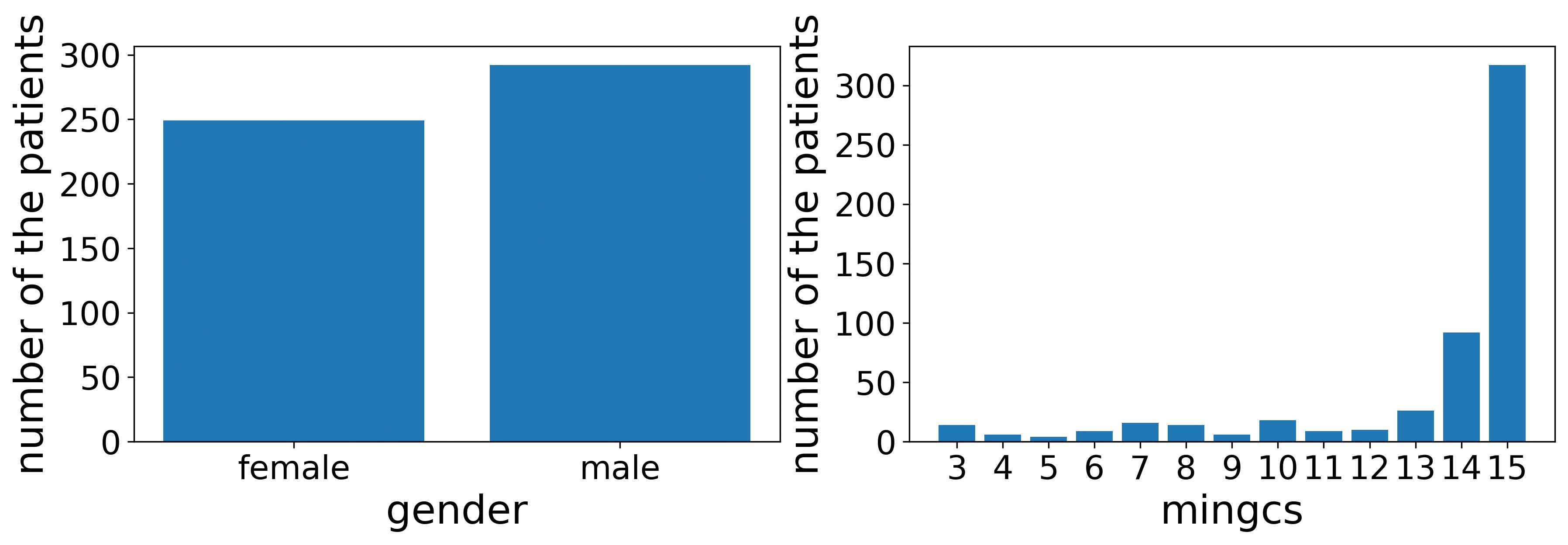
The data distribution histograms of discrete variables.

3.2. Prediction Results and Comparison

Table 1 shows the prediction results of different methods, including the MAE, 1st quartile and 3rd quartile. Our proposed model gets the lowest MAE when p equals 0.15. We choose two long sequences and describe the change of the real dose of norepinephrine and the prediction curves of different methods in Figure 10. The change of the real dose is drawn in the blue line. The red line, which is the prediction results of our proposed model, is a close fit to the blue line.

Model	MAE	1st Quartile	3rd Quartile
LSTM + dropout (p=0.15)	0.0260	0.0065	0.0303
Linear regression	0.0487	0.0174	0.0532
XGBoost regression	0.0388	0.0104	0.0398

MAE, mean absolute error; LSTM, long short-term memory.

Table 1

MAE for different models.

Figure 10

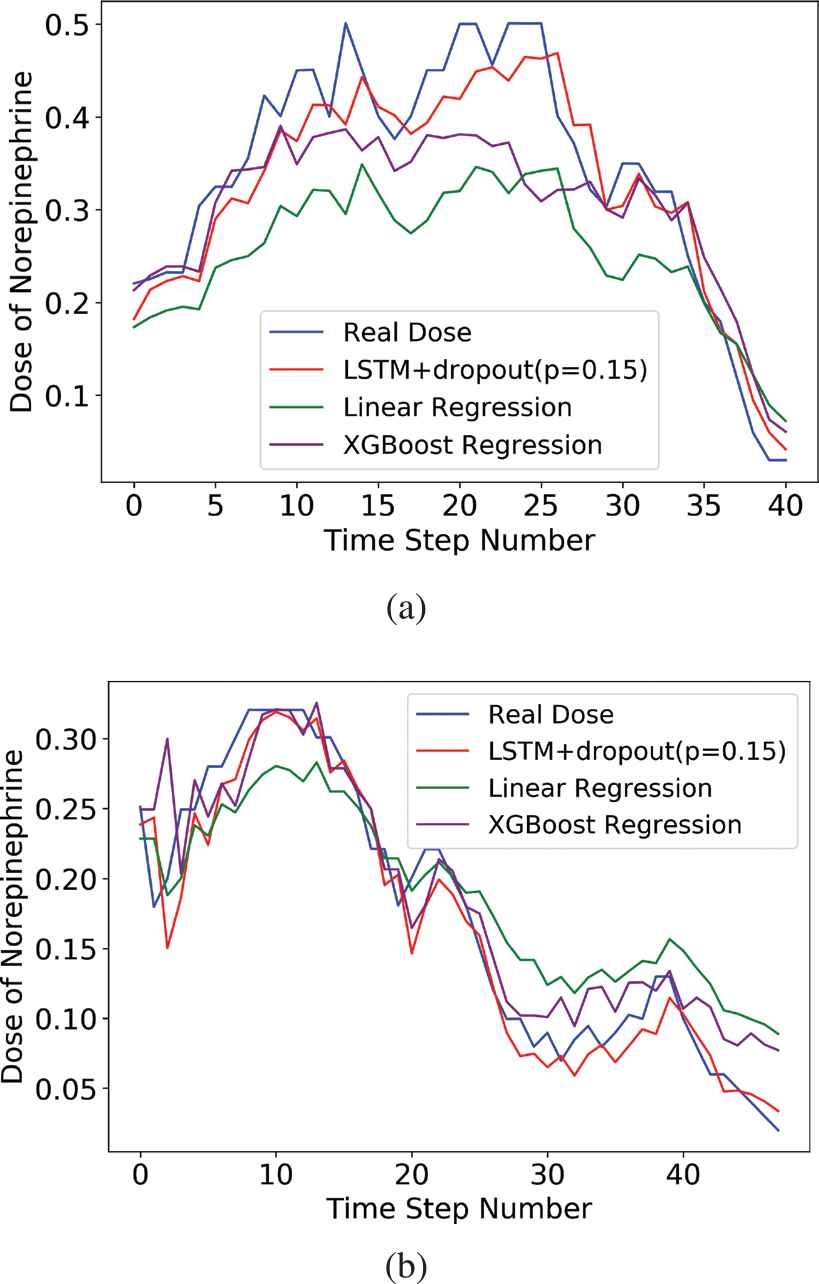
The change of the real dose of norepinephrine and the prediction curves of different methods.

3.3. Clustering Results and Analysis

After that, we cluster the data and judge whether cluster analysis can reduce the MAE. Figure 11 shows the variation of the silhouette coefficient of the clustering result with the number of the clusters K when using two different methods to measure the similarity of time series. We can see that for both methods, the clustering result is better when K=2. The visualization result by t-distributed Stochastic Neighbor Embedding (t-SNE) algorithm [31] for two different clustering results when K=2 is shown in Figure 12.

Figure 11

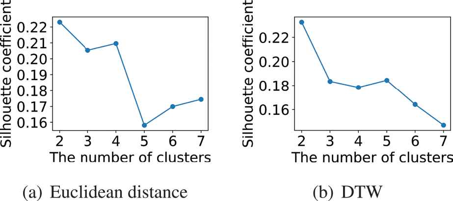
The silhouette coefficient of the clustering results with different value K when using two different methods to measure the similarity of time series.

Figure 12

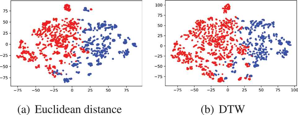
The visualization result by t-SNE algorithm for two different clustering results when K = 2.

Then we use the LSTM network shown in Figure 4 with different dropout probability p to predict the dose and calculate MAEtotal on the whole dataset with and without clustering. Results are shown in Table 2. When p=0.25, best MAEtotal are 0.0263 and 0.0267 respectively for different versions of k-means. When clustering is not used, the best MAEtotal is 0.0260 which is achieved with p=0.15. We can see that clustering cannot reduce the prediction error. Actually, the prediction results with and without clustering are very close.

Model	MAE	1st Quartile	3rd Quartile
K-means (Euclidean Distance)	0.0263	0.0072	0.0305
+ LSTM + dropout (p=0.25)
k-means (DTW)	0.0267	0.0070	0.0320
+ LSTM + dropout (p=0.25)
LSTM (without clustering)	0.0260	0.0065	0.0303
+ dropout (p=0.15)

MAE, mean absolute error; LSTM, long short-term memory; DTW, dynamic time warping.

Table 2

MAE_total with and without clustering.

4. DISCUSSION

Sepsis has been a major cause of death for many years in critically ill patients [32], especially to the patients with septic shock. As the initial target, MAP of 65 mmHg in patients with septic shock requiring vasopressors has been strongly recommended based moderated quality of evidence, and norepinephrine is one of the most important vasopressors [14], usually the first choice for medical treatment. We recognize that doctors and caregivers have to act quickly given the seriousness of sepsis that is even more impacted if the case is an emergency or when a doctor has a large case load and has to account for the dosage change may have for the prognosis of the patient. The focus of our research is to investigate the modeling approach to predict and adjust automatically the dose of norepinephrine for sepsis patients.

The dosage adjustment of norepinephrine may be related to many factors, such as disease severity, basic demographic information, fluid intake and outflow volume, heart and kidney function, complications, combined drug use and so on. Due to the limitation of information contained in the database and the reduction of complexity, we focus on sepsis patients who meet some criteria and eventually selected 14 dimensions information related to the development process of sepsis, including patient's basic information, vital signs and laboratory test results. Since the linear correlation among these dimensions that fit the normal distribution is quite weak, they would not be alterative that have individual difference with respect to dose prediction. We thus select these dimensions so that we can predict the dose more accurately based on all aspects of the patient's information. After filling in the missing values, we process the data into multidimensional time series data with the same length. The best length is selected by comparing the prediction results using a single layer LSTM network.

Considering the temporal data characteristics and the advantages of LSTM network in processing time series data, the LSTM network is used to predict the dose of norepinephrine in our work. The LSTM network structure in Refs. [6,8] has only one layer, and the learning ability may be weak. However, it is very easy to cause overfitting if the network is too deep, like the LSTM network with three recurrent layers in Ref. [7], because we only have 4119 time series data. So, we deepen the network structure and construct an LSTM network with two recurrent layers. Meanwhile, for the purpose of preventing overfitting when training models on smaller dataset after clustering, dropout mechanism is used between two recurrent layers.

From the prediction results shown in Table 1 and Figure 10, we can see our proposed method yields better results than two widely applicable baselines in the medical field, i.e., linear regression and XGBoost regression. The input of both linear regression and XGBoost regression is the data consisting of only one time step, and the input of LSTM network is time series data, which contains the changes of patient's data and the information related to temporal attributes that people cannot perceive intuitively. This might explain why the prediction result of our proposed model is superior to baselines. However, all of the prediction curves in Figure 10 have a certain hysteresis compared to the true value curve (the blue line), so whether this will affect the clinical effect remains to be verified.

In addition, we explore whether clustering analysis can help to achieve more accurate prediction by clustering data first and predicting based on the clustering results. The data is clustered according to the changes of patients' historical dose, vital signs and laboratory test results recorded in patient care including ca.10 time treatments. Two methods for measuring time series similarity, i.e., Euclidean distance and DTW, are used as part of k-means clustering. Then we check which cluster a patient's time series data is located. The result is shown in Table 3, where the three columns represent the number of patients whose time series data are located in cluster 0, cluster 1 or both clusters, respectively. From the result, we see that for most patients their time series data are located in either one of the two clusters, not both.

Since the dose data in the MIMIC-III database is adjusted manually by doctors, what our model does is to imitate doctors' behavior. When we continue to imitate the doctor's behavior based on the clustering results, actually the predicted results are not obviously improved, as shown in Table 2. The reason is that at the stage of being there is no clinical segmentation of sepsis patients according to their vital signs and disease development. This also exposes the shortcomings of clinical segmentation, which makes doctors adopt the same treatment strategy for different patient groups. So, through the analysis of the correlation between different dimensions and the difference between the prediction results before and after clustering, our work may provide some enlightenment for doctors to further lean treatment in the future.

5. CONCLUSION

In this paper, we analyze the medical time series data by AI techniques to predict the dose of norepinephrine. It has shown that the proposed modeling approach resulted in lower MAE than other learning methods, achieving better performance in dosage prediction. The proposed approach can be used to build a solution that may automatically set the dose of norepinephrine for individual patients, help doctors treat patients in sepsis, reduce the workload of doctors and caregivers, and improve the prognosis for patients. Moreover, we further explored the possibility of clustering patients for prediction helpful to improve the effects on dose adjusting. The future work is considered not only to imitate the doctor's behavior, but also to adjust the dosage for assisting the doctor's medical treatment according to the patient's pathophysiology, the development of the disease and the law of response to the drug.

CONFLICT OF INTEREST

The authors declare no conflict of interests.

AUTHORS' CONTRIBUTIONS

J. Liu, W. Guo. designed the experiments and provided the clinical expertise and context; M. Gong, C. Li preprocessed the data, implemented the prediction model based on LSTM and clustering algorithms; H. Wang, S. Zhang, C. Nugent contributed to analyses of the data and updates of the manuscript.

Funding Statement

This research work was supported by China NSF Project under Grant No. 61672309 and the Royal Society International Exchanges Award (IE161780).

ACKNOWLEDGMENTS

We gratefully acknowledge the helpful discussions with Peter Nicholas for proofreading the manuscript.