
Optimizing Production Mix Involving Linear Programming with Fuzzy Resources and Fuzzy Constraints
 , Z. Wang3, O.V. Samakin4, , S. Wu5, X. Liu3
- DOI
- 10.2991/ijcis.d.200519.002How to use a DOI?
- Keywords
- Fuzzy resources; Fuzzy constraints; Fuzzy objective function; Fuzzy optimization
- Abstract
In this paper, Fuzzy Linear Programming (FLP) was used to model the production processes at a university-based bakery for optimal decisions in the daily productions of the bakery. Using the production data of five products from the bakery, a fuzzy linear programme was developed to help make decisions when fuzzy resources were involved. As usual, classical linear programme gave only one feasible solution. However, while it was established that solving the linear programme from the production mix when fuzzy constraints were introduced (Verdegay's model) gave a more robust and alternative set of decisions than the classical model, it was equally established that a better result could be obtained when all the constraints and the objective function were fuzzy (Werners' Model).
- Copyright
- © 2020 The Authors. Published by Atlantis Press SARL.
- Open Access
- This is an open access article distributed under the CC BY-NC 4.0 license (http://creativecommons.org/licenses/by-nc/4.0/).
1. INTRODUCTION
Linear Programming (LP) has its origin during the second world war (1939-1945) when a balance between man and material (resources) had to be maintained. Hence, LP was developed in order to plan expenditures and returns to reduce costs of the army and increase losses imposed on the enemy. During that time, Marshall K. Wood worked on the allocation of the resources for the United States and methods were developed to allocate resources in such a way that will minimize or maximize the desired objective of the problems as the case may require. As time went on, economists formulated classical economic problems, transportation problems and assignment problems. Then the simplex method of solving linear programmes was introduced by George B. Dantzig [1] which, for the first time, efficiently tackled the LP problem in most cases. Many industries found the use of LPvaluable, hence, accelerating its development.
LP is the mathematical technique which involves the use of limited resources in an optimal manner. LP problems requiring such judicious use of resources are called optimization problems. In such classical optimization problems, a solution which is feasible is the goal.
It is also important to note that optimization has gone beyond allocating resources. Various optimization methods have also been developed to solve problems that occur in other physical sciences. Some of such can be found in [6,5,12,15,17,18] just to mention a few.
Most of the traditional tools for formal modeling, reasoning and computing are precise in nature, that is, they are the yes-or-no type and not more-or-less type. Unfortunately, many real life problems encountered from time to time suggest the need for more robust mathematical tools. Take, for an instance, if an investor hopes to make profit “around” an amount using “not more” than “around certain quantity” of raw materials, the usual LP method cannot model the situation properly. This is as a result of the vague language “around” which introduces uncertainty into the problem. Also, to be able to develop model which classifies goods and services as being “expensive” or “affordable” and the like, it is necessary for the existence of a mathematical modeling of vague knowledge to capture elements that cannot be precisely said to be in a set or not but are in between.
Mathematical study of vagueness of this sort (fuzzy sets) began with a professor of electrical engineering, Lofti A. Zadeh, in the University of California at Berkeley, when he published the first paper Fuzzy Sets in 1965 [20]. In it, he noted that “The notion of a fuzzy set provides a convenient point of departure for the construction of a conceptual frame-work which parallels in many respects the framework used in the case of ordinary sets, but is more general than the latter and, potentially, may prove to have a much wider scope of applicability, particularly in the fields of pattern classification and information processing. Essentially, such a framework provides a natural way of dealing with problems in which the source of imprecision is the absence of sharply defined criteria of class membership rather than the presence of random variables.”
Fuzzy set theory provides a mathematical framework in which vague conceptual phenomena can be rigorously studied. It can also be considered as a modeling language well suited for situations in which fuzzy linguistic variables such as “much,” “very much,” “high,” “very high” and the like occur. Zadeh and others continued to develop the fuzzy logic at that time. The idea of fuzzy sets and fuzzy logic, though were not well accepted then, have now been extended to many areas of discipline and studies.
Extension of fuzziness to LP has led to Fuzzy Linear Programming (FLP) in which some of the parameters constitute fuzzy set(s). One case is to have a crisp objective but fuzzy constraints. Another case is to have a fuzzy objective but crisp constraints. However, it is also possible to have a FLP in which both the constraints and the objective are fuzzy. Precisely, in this paper, an approach used by [4], crisp objective but fuzzy constraints, is improved on.
2. PRELIMINARIES
Definition 1.
[20] A fuzzy set
Definition 2.
[20] The support of a fuzzy set
Definition 3.
([20] A fuzzy set
Definition 4.
([20] Two fuzzy sets
Definition 5.
[20] A fuzzy set
Definition 6.
[20] The intersection of two fuzzy sets
Definition 7.
[20] The union of
Definition 8.
[20] If
3. LINEAR PROGRAMMING
A LP is an optimization problem in which the objective function and constraints are given as mathematical functions and functional relationships. Linear programmes are of the form
The programme attempts to find the best solution, called an optimal solution, for a problem under consideration. It seeks to find values of the decision variables that optimize (that is, maximize or minimize) an objective function among a set of values.
Solving LP by simplex method according to [1] involves using matrix procedures to solve standard LP of the form
In what follows,
| A | B | |
|---|---|---|
Simplex table for minimization programmes.
| A | B | |
|---|---|---|
Simplex table for maximization programmes.
4. METHODOLOGY: FLP
In FLP, the fuzziness of available resources is characterized by the membership function over the tolerance range. Then, the membership function of the optimal solutions is constructed by the convolution of the membership function of the constraints. The general model of linear programmes with fuzzy resources is
Verdegay's Approach—A Nonsymmetric Model: Verdegay in [19] considered that the membership functions of the fuzzy constraints in (5) are
Furthermore, if these
In the membership functions, the degree of satisfaction of the constraints is depending on whether
Now, the membership function of (6) is substituted into (7) to get a parametric programme.
But, further than having a FLP with fuzzy constraints, the objective function can altogether be made fuzzy and the results of these two can be compared.
Werners' Approach—A Nonsymmetric Model [16]: Given the linear programme with fuzzy resources
Werners proposed that the objective function of Equation (9) should be fuzzy because of fuzzy total resources or fuzzy inequality constraints. Let it be assumed that the tolerances
Thus, a continuously nondecreasing linear membership function can be constructed for the objective function by use of
With the above membership function, the max-min operator can be used to obtain optimal decision. Then, Equation (9) can be solved by solving
5. RESULTS AND DISCUSSION
The data used in this study was collected from an institution-based bakery. The production data of five different kinds of bread stated below was used for the purpose of this project. The linear programme was solved, using the Simplex method to get the crisp optimal solution.
Furthermore, fuzzy elements were introduced to the resources and the new Fuzzy linear programme was solved using the Verdegay's Approach—A Nonsymmetric Model, where only constraints were fuzzy. Then, the Werners' Approach—A Nonsymmetric Model, where both the objective function and the constraints were fuzzy was also applied to the data. The results of the Classical Linear Programme and these Fuzzy linear Programmes were compared.
Products Considered: Let
Chocolate bread
Coconut bread
White bread
Note also,
From the data collected, the bakery made a profit of
| Bread Kind | Flour | Sugar | Salt | Butter | Unit Profit |
|---|---|---|---|---|---|
| Chocolate | |||||
| Coconut | |||||
| White | |||||
| Available resources | Maximize |
The input data for the Bakery problem.
5.1. Obtaining Crisp Solution
The associated linear programme is
From the simplex table we have the crisp optimal solution
The actual resources used are
5.2. Obtaining Fuzzy Solution When Only Some Constraints are Fuzzy
Given that the flour used has a tolerance of
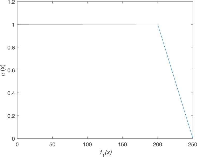
The membership function of flour constraint.
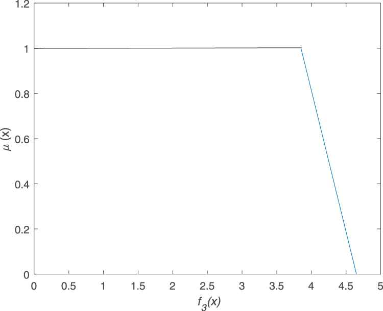
The membership function of salt constraint.
For salt,
The fuzzy linear programme of (14) is
The solutions of the FLP (18) is given in the Table 4 below.
| 0.00 | 51828.52 | 200.00 | 11.91 | 3.19 | 1.00 |
| 0.10 | 52910.00 | 205.00 | 12.20 | 3.27 | 1.00 |
| 0.20 | 53991.43 | 210.00 | 12.50 | 3.35 | 1.00 |
| 0.30 | 55072.66 | 215.00 | 12.80 | 3.43 | 1.00 |
| 0.40 | 56154.29 | 220.00 | 13.06 | 3.51 | 1.00 |
| 0.50 | 57235.71 | 225.00 | 13.39 | 3.59 | 1.00 |
| 0.60 | 58317.14 | 230.00 | 13.69 | 3.67 | 1.00 |
| 0.70 | 59398.57 | 235.00 | 13.99 | 3.75 | 1.00 |
| 0.80 | 60480.00 | 240.00 | 14.29 | 3.83 | 1.00 |
| 0.90 | 61561.43 | 245.00 | 14.58 | 3.91 | 1.00 |
| 1.00 | 62642.86 | 250.00 | 14.88 | 3.99 | 1.00 |
The solutions of the fuzzy liner programing (FLP) (18).
5.3. Obtaining Fuzzy Solution When Both the Objective Function and All Constraints are Fuzzy
From the crisp LP problem in (14), it can be seen that
Setting
Then, solving Equation (11),
The problem is actually equivalent to
6. COMPARISON OF RESULTS
As can be seen from Section 5.1, using the classical LP produced one feasible point
The result of Verdegay's model can be seen in Table 4, giving various optimal points inclusive of the one obtained by classical LP. More importantly, the result of Werner's model can be seen in Table 5. It also gave as many optimal solutions as the Verdegay's model but, with as much resources as used under Verdegay's model, it gives greater profit margin.
| 0.00 | 51828.52 | 200.00 | 11.91 | 3.19 | 1.00 |
| 0.10 | 53081.40 | 205.00 | 12.20 | 3.27 | 1.02 |
| 0.20 | 54334.28 | 210.00 | 12.50 | 3.35 | 1.04 |
| 0.30 | 55587.17 | 215.00 | 12.80 | 3.43 | 1.06 |
| 0.40 | 56840.05 | 220.00 | 13.06 | 3.51 | 1.08 |
| 0.50 | 58092.93 | 225.00 | 13.39 | 3.59 | 1.10 |
| 0.60 | 59345.81 | 230.00 | 13.69 | 3.67 | 1.12 |
| 0.70 | 60598.70 | 235.00 | 13.99 | 3.75 | 1.14 |
| 0.80 | 61851.58 | 240.00 | 14.29 | 3.83 | 1.16 |
| 0.90 | 63104.46 | 245.00 | 14.58 | 3.91 | 1.18 |
| 1.00 | 64357.34 | 250.00 | 14.88 | 3.99 | 1.20 |
The solutions of the fuzzy linear programing (FLP) (26).
7. CONCLUSIONS
The study has revealed that, using FLP gives a more robust information on making decision. More importantly, it has also shown that, with almost the same resources, modeling production mix with both the objective function and the constraints being fuzzy yields a better result and can enhance better performance and production output more than crisp modeling and modeling with only the resources being fuzzy.
CONFLICT OF INTEREST
The authors declare that there are no conflicts of interest.
AUTHORS' CONTRIBUTIONS
All the authors have contributed fairly well.
ACKNOWLEDGMENTS
This work is supported by Foundation of Chongqing Municipal Key Laboratory of Institutions of Higher Education ([2017]3), Foundation of Chongqing Development and Reform Commission (2017[1007]), and Foundation of Chongqing Three Gorges University.
REFERENCES
Cite this article
TY  - JOUR
AU  - B.O. Onasanya
AU  - Y. Feng
AU  - Z. Wang
AU  - O.V. Samakin
AU  - S. Wu
AU  - X. Liu
PY  - 2020
DA  - 2020/06/11
TI  - Optimizing Production Mix Involving Linear Programming with Fuzzy Resources and Fuzzy Constraints
JO  - International Journal of Computational Intelligence Systems
SP  - 727
EP  - 733
VL  - 13
IS  - 1
SN  - 1875-6883
UR  - https://doi.org/10.2991/ijcis.d.200519.002
DO  - 10.2991/ijcis.d.200519.002
ID  - Onasanya2020
ER  -