
An Efficient Clustering Algorithm for Mixed Dataset of Postoperative Surgical Records
 , Rinkle Rani
- DOI
- 10.2991/ijcis.d.200601.001How to use a DOI?
- Keywords
- Data clustering; Meta-heuristic; Artificial electric field algorithm; Distance measure; Mixed dataset
- Abstract
In data mining, data clustering is a prevalent data analysis methodology that organizes unlabeled data points into distinct clusters based on a similarity measure. In recent years, several clustering algorithms found, dependent on a predefined number of clusters and centered around the dataset with either numeric or categorical attributes only. However, many real-world engineering, scientific, and industrial applications involve datasets with mixed numeric as well as categorical attributes but lack domain knowledge (target labels). Clustering unlabeled-mixed datasets is a challenging task as (1) it is difficult to estimate the number of clusters in the absence of domain knowledge and (2) mathematical operations cannot be applied directly to the mixed dataset. In this paper, an efficient searching and fast convergent automatic data clustering algorithm based on population-based meta-heuristic optimization is proposed to deal with the mixed dataset. The proposed clustering algorithm aims to find the optimal number of cluster partitions automatically. It utilizes a real-coded variable-length candidate solution to detect the optimal number of clusters automatically. The concepts of threshold setting and cut-off ratio are used in the optimization process to refine the clusters. The similarity between data points and different cluster centers is measured using Euclidean distance (for numeric attributes) and the probability of co-occurrence of values (for categorical attributes). The proposed algorithm is compared with existing mixed data clustering techniques based on a statistical significance test and two robustness measures: Average accuracy and Standard deviation. Finally, the proposed algorithm is validated by applying to a real historical postoperative surgical mixed data set obtained from a surgical department of a multispecialty hospital in India. Results show the effectiveness, robustness, and usefulness of the proposed clustering algorithm.
- Copyright
- © 2020 The Authors. Published by Atlantis Press SARL.
- Open Access
- This is an open access article distributed under the CC BY-NC 4.0 license (http://creativecommons.org/licenses/by-nc/4.0/).
1. INTRODUCTION
Data clustering is a data analysis approach that arranges unlabeled data into different groups based on a similarity measure. Each group is called a “cluster,” which shows similarity among the data in it and differs from the set of data in other clusters. Clustering is most widely used in those disciplines where multivariate data analysis is required. In recent years, cluster analysis has played a significant role in the distinct domains of various fields such as engineering, life, and medical sciences, earth sciences, and economics [1–3]. The elementary problem of the clustering analysis is to accurately determine the approximate number of clusters, as this number influences the clustering outcomes to a large extent [4]. Clustering algorithms are classified into two main categories: partitional clustering [5] and hierarchical clustering [6]. The hierarchical clustering arranges data points in a hierarchical tree structure based on the homogeneity among the data points. It overlooks the shape and size of the formed clusters. Further, this clustering allocates a single cluster to a data point at a time that renders the cluster structure static. Contrary, partitioning clustering analyzes the dataset and organizes data points into clusters based on the similarity among data points. The partitioning clustering aims to optimize a global criterion involving minimizing the similarity among the elements within a cluster and maximizing the disparity between different clusters. Although both of these algorithms prove their usefulness and performance in various domains, both still have some critical limitations. The efficacy of these algorithms depends on the foreknowledge of the number of clusters present in the datasets. Since different datasets, especially in real-world applications, have diverse patterns, cluster analysts lack information on how many appropriate clusters exist in the dataset [7]. Hence, these algorithms that require the cluster number as an onset parameter cannot be used effectively. Since most real-world datasets do not have class labels, there are no specific criteria for directing clustering analysis. It is considered a major limitation [4] of the dataset, which makes it a challenging task to find a suitable number of clusters. Therefore, determining the optimum number of clusters in a data set has become an essential research issue to address such limitations. In recent years, the concept of the automatic clustering method has been used to overcome this limitation in clustering. Automatic clustering is defined as an analytic process of determining a suitable number of clusters in the dataset, irrespective of any prior knowledge related to the dataset [8]. Several automatic clustering algorithms, mostly inspired by natural phenomena, involving genetic algorithm (GA) [9,10], particle swarm optimization (PSO) [11,12], gravitational search algorithm (GSA) [13,14], differential evolution (DE) [15], bacterial evolutionary algorithm (BEA) [16], and bee colony optimization algorithm (BCA) [17,18], etc., are introduced in recent years. In these algorithms, clustering is considered as an optimization activity, aiming to maximize the similarity among the data of a cluster and maximize the disparity among disjoint clusters [19] . These algorithms have proven their higher convergence speed and efficacy in producing quality outcomes not only in optimization but also in clustering analysis. In this paper, clustering analysis is framed as an optimization problem, and an efficient clustering algorithm based on a meta-heuristic optimization algorithm, called Artificial Electric Field Algorithm (AEFA) [20], is proposed to address the automatic clustering problem. AFEA is a recent inclusion in the global pool of population-based meta-heuristic algorithms that contributes to global optimization. To the extent of our knowledge, there is no such contribution where AEFA has been employed for automatic clustering analysis. The proposed clustering algorithm attempts to address two issues. The first is to select the optimal clusters automatically, and the second is to focus on mixed datasets with numerical as well as categorical attributes contrary to recent studies that focus on data set with either numerical or categorical datasets only. AEFA simulates the Coulomb’s law of attraction electrostatic force and law of motion. Traditional AEFA begins with an initial population of charged particles (candidate solutions). During the optimization process of AEFA, the fitness of each charged particle is computed that helps in determining the charges and forces on each charged particle, which further enables the global movement of all charged particles toward a heavier charged particle. Finally, a particle with heavier charge is selected as a globally optimum solution. Similarly, in the proposed clustering algorithm, the initial population of charged particles is formed by selecting a set of random cluster centers from the dataset where each charged particle is encoded using a real-coded variable-length encoding approach. The fitness of each charged particle is computed using a fitness function based on the SD index [21]. The probability of co-occurrence of value for categorical attributes along with Euclidean distance for numeric attributes is used as a distance measure for assigning the data points to a particular cluster. The optimization process is carried out until the optimum clusters are obtained.
1.1. Our Contribution
An efficient data clustering algorithm for the mixed dataset based on population-based meta-heuristic is proposed.
The concepts of threshold setting and cut-off ratio are used in the optimization process to refine the clusters.
The proposed algorithm is evaluated on real-life datasets and compared with existing mixed dataset clustering techniques. Further, it is also validated using the real postoperative surgical dataset of a multispecialty hospital.
This paper is organized in the following way: Section 2 covers an overview of the existing literature on clustering analysis; Section 3 describes the preliminaries and background algorithms; Section 4 describes the proposed clustering algorithm in detail; Section 5 presents results and performance of the proposed algorithm in comparison to existing clustering techniques; Section 6 sums up the findings and discuss the future work of this research in concluding remarks.
2. RELATED WORK
K-means is a center-based clustering approach widely used in the partitioning of the data set for its simplicity and efficacy. The major drawback of the k-means algorithm involves its dependency on an initial number of the cluster centers and its faster convergence to the local optima [22,23]. Although several clustering algorithms [24–26] have been proposed to prevent solution from being stuck in the local optima, still the reliance of the algorithm on prior cluster number information and its adverse effect on clustering performance has emerged as an issue [27–30]. For addressing such an issue, several optimization algorithms have been adapted to implement automatic clustering analysis. The first-ever contribution toward automatic clustering was based on evolutionary computing, called EP-clustering [31]. EP-clustering was aimed to minimize the DB index and WGS indices for improving the efficiency of exploration and exploitation. This algorithm produced better results as compared K-means algorithm when implemented on real-life datasets. In recent years, Chen et al. [32] introduced a GEP-cluster algorithm based on gene expression [33] programming for the automatic clustering of data. GEP-cluster comprised of clustering algebra as a new concept for identifying the best cluster with no prior knowledge, and an automatic merging clustering algorithm for merging clusters automatically. The results indicated that the GEP-cluster algorithm is found noise sensitive as well as incompetent to high-dimensional datasets. Lee and Antonsson [34] introduced evolutionary strategy-based clustering, also called, ES-clustering for automatic clustering of data. In ES-clustering, the initial population is encoded using genomes of variable-length and
| Author(s) | Objective/Work Done | Technique Proposed/Used | Performance Parameters | Research Gap(s) |
|---|---|---|---|---|
| Liu et al. [7] | The author proposed an automatic clustering algorithm based on the genetic algorithm | Automatic genetic clustering for unknown K (AGCUK) |
|
The algorithm is limited to either numeric or categorical datasets only |
| Kumar et al. [13] | The author proposed an automatic data clustering using an adaptive harmony search algorithm (AHSA) | Adaptive harmony search algorithm (AHSA) |
|
The algorithm is limited to numeric attributes only |
| Kumar and Kumar [14] | The author proposed an automatic data clustering and feature selection using the gravitational search algorithm (GSA) | Automatic clustering and feature selection using gravitational search algorithm (GSA_CFS) |
|
The algorithm is limited to either numeric or categorical datasets only |
| Das et al. [15] | The author proposed an automatic clustering algorithm using an improved differential evolution algorithm | Automatic clustering DE algorithm (ACDE) |
|
The algorithm is limited to either numeric or categorical datasets only |
| Das et al. [16] | The author proposed an automatic clustering algorithm based on the bacterial evolutionary approach | Automatic clustering using the bacterial evolutionary algorithm (ACBEA) |
|
The algorithm is limited to either numeric or categorical datasets only |
| Sarkar et al. [31] | The author proposed data clustering based on evolutionary programming | EP-clustering | DB-Index | This algorithm is sensitive to the initial cluster number. Further, this algorithm is limited to numeric attributes only |
| Chen et al. [32] | The author proposed an automatic clustering algorithm based on gene expression programming |
|
|
This algorithm is sensitive to noise and found efficient for high dimensional data |
| Lee and Antonsson [34] | The author proposed a dynamic clustering algorithm based on evolutionary strategy approach | Evolutionary strategy-based clustering (ES-clustering) | Heuristic mean square error | The efficacy of the proposed algorithm is not tested on high-dimensional data |
| Tseng and Yang [35] | The author proposed an automatic clustering algorithm using genetic algorithm and heuristic strategy | CLUSTERING | The average distance from the cluster center | The algorithm did not focus on mixed datasets |
| Bandyopadhyay and Saha [37] | The author proposed a point symmetry-based genetic clustering algorithm for automatic portioning of data | Variable-length point symmetry-based genetic clustering algorithm (VGAPS) |
|
This algorithm is focused on point-based symmetry only. Further, the algorithm is limited to either numeric or categorical data only |
| Ahmad and Dey [38] | The author proposed K-mean clustering algorithm for the mixed data type | K-mean clustering for mixed dataset (KMCMD) |
|
The cluster center initialization problem persists |
| Chang et al. [40] | The author proposed an automatic clustering algorithm based on dynamic niching and niche migration | Dynamic niching and niche migration clustering (DNNM-Clustering) |
|
The algorithm is sensitive to the size of the initial population |
| Pan and Cheng [41] | The author proposed a framework for automatic clustering algorithm based on tabu search and genetic operators | An evolution-based tabu search approach (ETSA) | Cluster validity index (PBM-index) value | The algorithm is limited to either numeric or categorical datasets only |
| Cura [45] | The author proposed a data clustering algorithm using enhanced particle swarm optimization (PSO) | Enhanced particle swarm optimization-based clustering (EPSO-clustering) |
|
Robustness decreases when dealing with problems where the numbers of clusters are unknown |
| Chowdhury et al. [46] | The author proposed an automatic clustering based on invasive weed optimization (IWO) algorithm | IWO-clustering | Minkowski score | The algorithm is limited to either numeric or categorical datasets only |
Summary of existing clustering methods.
3. PRELIMINARIES AND BACKGROUND
This section briefly discusses the basic concepts of partitioning clustering, AEFA, and the distance measure for the mixed dataset.
3.1. Partitioning Clustering
Partitioning clustering is a data clustering approach that groups the data points into disjoint clusters. Let us consider a dataset
3.2. Distance Measure for Mixed Datasets
The belonging of a data point to a cluster is measured using the distance computed between the cluster and data point. Distance measure ensures the similarity among the data points belonging to the same cluster and dissimilarity between disjoint clusters. Grouping a mixed dataset into clusters is a significantly challenging task. It requires a suitable distance measure, which can compute the similarity/dissimilarity between data points effectively, to be involved in the clustering process. In this paper, the distance measure proposed by Ahmad and Dey
3.3. Artificial Electric Field Algorithm
AEFA 20 is a population-based meta-heuristic, which mimics the Coulomb’s law of attraction electrostatic force and law of motion. In AEFA, the possible candidate solutions of the given problem are represented as a collection of the charged particles. The charge associated with each charged particle helps in determining the performance of each candidate solution. Attraction electrostatic force causes each particle to attract toward one another resulting in the global movement toward particle with the heavier charge. A candidate solution to the problem corresponds to the position of charged particles and fitness function, which determines their charge and unit mass. The steps of AEFA are as follows:
Step 1. Initialization of population: A population of P candidate solutions (charged particle) is initialized as follows:
Step 2. Fitness evaluation:Performance of each charged particle depends on the fitness values at each iteration. The best and worst fitness is computed as follows:
Step 3. Computation of Coulomb’s constant: At time t, the Coulomb’s constant is denoted by
Step 4. Compute the charge of charged particles: At time
Step 5. Compute the electrostatic force and acceleration of the charged particles:
The electrostatic force exerted by
where
The acceleration
where
Step 6. Updation of velocity and position of charged particle:At time
4. PROPOSED CLUSTERING ALGORITHM
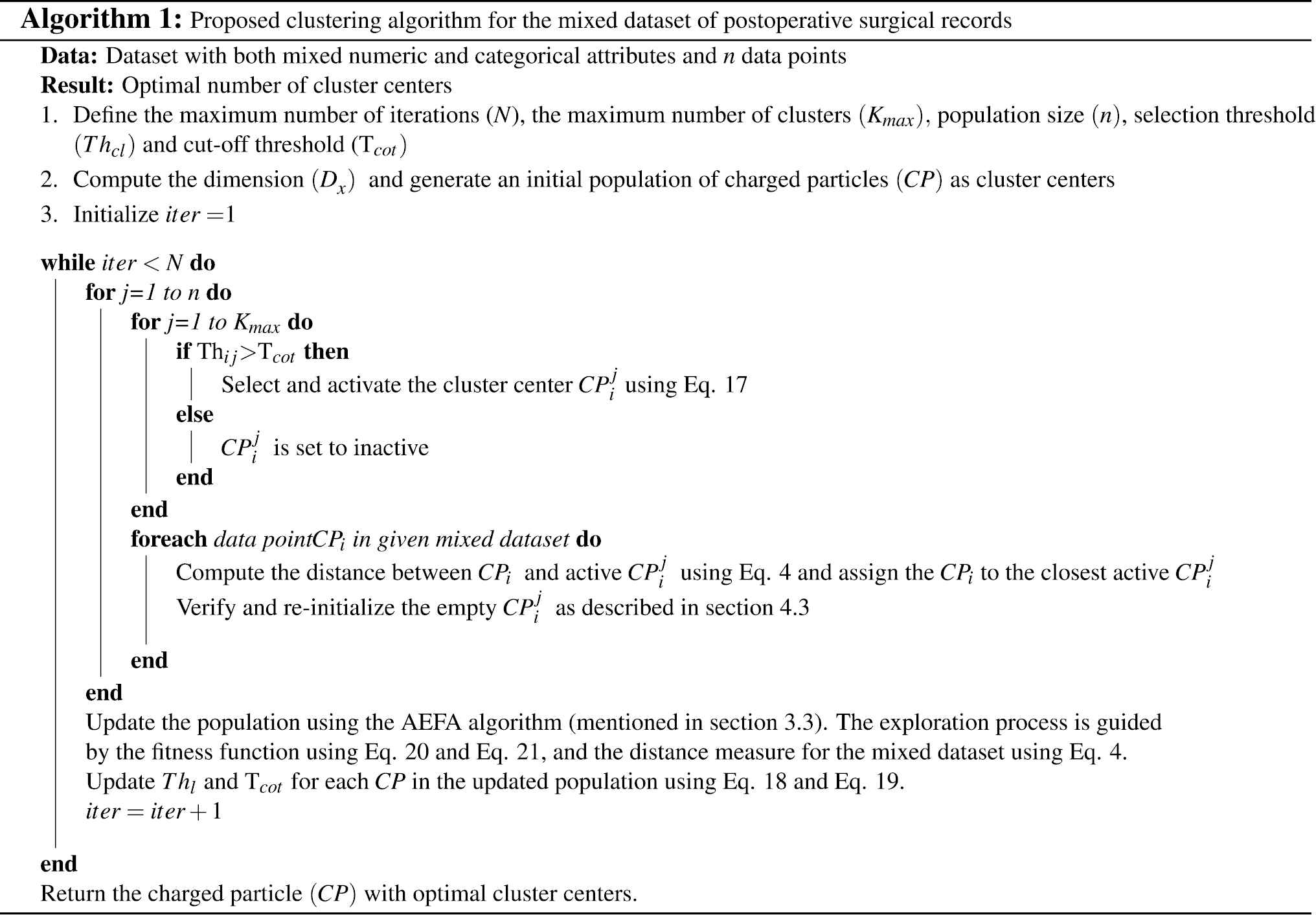
In this section, the proposed clustering algorithm is described in detail. The algorithm starts with accepting pre-processed mixed dataset as input and initializes parameters. Then, a population of candidate solutions is generated, where each solution composed of two segments: the first segment represents threshold values and the second segment represents cluster centers. The threshold values of the first segment determine whether or not the corresponding cluster centers are active in the second segment. Further, by computing fitness value for each candidate solution, the best solution is selected. The population is iteratively updated until the termination conditions are satisfied, and the optimal solution is returned. The symbols used in the proposed algorithm are presented in Table 2. The detailed workflow and pseudocode of the proposed clustering algorithm are presented in Figure 1 and Algorithm 1, respectively.
| Symbol | Definition | Symbol | Definition |
|---|---|---|---|
| Distance between the data point and cluster center | Acceleration of |
||
| Electric field of |
|||
| Mass of |
|||
| Position of |
Velocity of |
||
| Maximum number of clusters centers | |||
| Dimension of objective space that helps in determining the overall dimension of a candidate solution | Population size (number of data points) | ||
| Objective fitness function | Overall dimension of a charged particle (candidate solution) | ||
| Best (lowest value for minimization problem and highest value for maximization problem) fitness value at time |
Maximum number of iterations | ||
| Worst (highest value for minimization problem and lowest for maximization problem) fitness value at time |
Threshold value of |
||
| Initial value for coulomb’s constant | The selection threshold value of a cluster center | ||
| Coulomb’s constant at time |
The cut-off threshold value of a cluster center | ||
| Small value of charge on |
SD index value of a |
||
| Total charge on a |
Intra-cluster distance of a |
||
| Force exerted by |
Inter-cluster distance a |
||
| Net force on |
Variance of clusters belonging to |
||
| Global best position of |
Variance of dataset |
||
| Current position of |
Maximum distance between the cluster centers of a charged particle | ||
| Distance between |
Minimum distance between the cluster centers of a charged particle | ||
| Total number of active clusters |
Symbols used in the proposed algorithm.
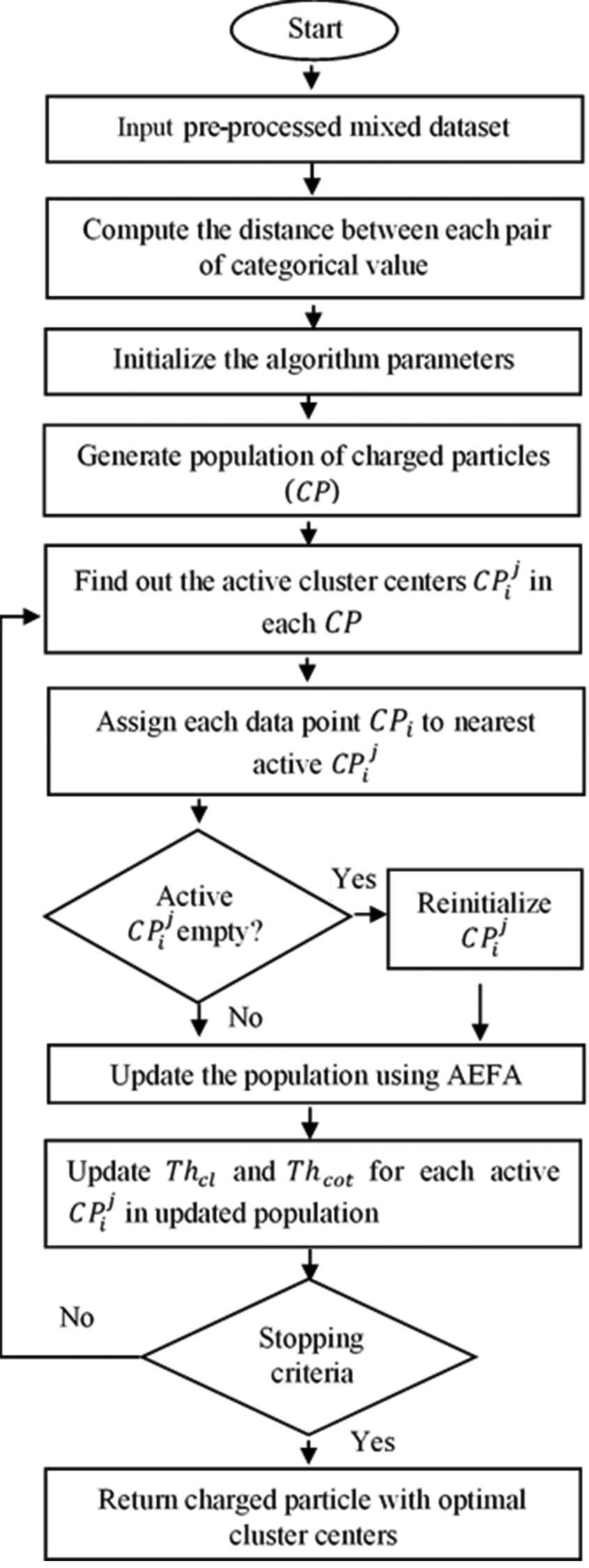
The workflow of the proposed clustering algorithm.
4.1. Population Generation
In this step, the population of candidate solutions is initialized. For the dataset, which has
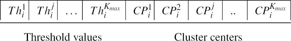 where
where 4.2. Active Cluster Center Selection
In this step, active cluster centers among
4.3. Empty Clusters Validation
A cluster center is said to be empty if no data points or less than 2 data points are assigned to it. Such problems are resolved by reinitializing the cluster center for that candidate solution. The candidate solution is reinitialized by assigning
4.4. Fitness Evaluation
In this step, the performance of the candidate solutions (cluster centers) is measured. As the performance critically relies upon a suitable cluster validation criterion. A random selection of criteria for clustering may lead to poor results. Therefore, the SD index
Here,
5. EXPERIMENTAL RESULTS AND DISCUSSION
This section is further divided into three subsections. Subsection 5.1 gives a performance comparison of the proposed algorithm with the existing mixed data clustering algorithms. Subsection 5.2 discusses the application of the proposed algorithm to the clustering of postoperative surgical records and Subsection 5.3 presents the statistical significance test of the proposed clustering algorithm.
5.1. Performance Comparison of the Proposed Clustering Algorithm with Existing Mixed Data Clustering Algorithms
At first, 5 real-life datasets are used to evaluate the performance of the proposed clustering algorithm. These datasets are obtained from the UCI machine learning repository https://archive.ics.uci.edu/ml/datasets.php). The description of the datasets is shown in Table 3. Then, the performance of the proposed clustering algorithm is compared with existing mixed dataset clustering algorithms. For performance comparison, two cluster quality measures average accuracy [38] and standard deviation [38] are used in this paper. Average accuracy represents the quality and the standard deviation represents the reliability of the clustering algorithm. During each iteration of the proposed clustering algorithm, both average accuracy and standard deviation contribute to the robustness of the clustering algorithm, where a high value of average accuracy and lower standard deviation makes a clustering algorithm more robust.
| Dataset | Data Points | Attributes |
Classes | |
|---|---|---|---|---|
| Numeric | Categorical | |||
| Heart Disease 1 | 303 | 5 | 8 | 2 |
| Heart Disease 2 | 270 | 6 | 8 | 5 |
| Credit approval | 690 | 6 | 8 | 2 |
| Iris | 150 | 4 | − | 3 |
| Soybean | 47 | − | 35 | 4 |
Characteristics of the real-life datasets.
5.1.1. Parameter setting
For experiments, the parameters used in the proposed clustering algorithm, i.e., population size (
5.1.2. Performance comparison
The performance of the proposed clustering algorithm is compared with existing mixed data clustering algorithm: K-means clustering algorithm for mixed dataset [38], and K-harmonic means clustering algorithm for the mixed dataset (KHMCMD) [39], K-prototype (KP) clustering for mixed data1 [47], improved K-prototype (IKP) clustering algorithm for mixed data [48], SBAC [49], and Ji et al. [50] The experiments are performed in 50 iterations. In every 10 iterations, the number of correct predictions of data points and corresponding class labels obtained by the proposed algorithm are computed in terms of average accuracy (
| Proposed Algorithm |
Improved K-prototype |
K-Prototype |
SBAC |
KHMCMD |
KMCMD |
Ji et al. [50] |
||||||||
|---|---|---|---|---|---|---|---|---|---|---|---|---|---|---|
| Dataset | ||||||||||||||
| Heart Disease (1) | 0.846 | 0.14 | 0.826 | 0.577 | 0.752 | 0.840 | 0.15 | 0.8389 | 0.15 | 0.808 | ||||
| Heart Disease (2) | 0.828 | 0.18 | 0.653 | 0.546 | 0.545 | 0.816 | 0.33 | 0.8074 | 1.20 | |||||
| Credit approval | 0.862 | 0.11 | 0.779 | 0.562 | 0.555 | 0.852 | 0.38 | 0.8223 | 12.77 | 0.794 | ||||
| Iris | 0.92 | 0.18 | 0.822 | 0.819 | 0.373 | |||||||||
| Soybean | 0.91 | 0.16 | 0.90 | 0.856 | 0.617 | |||||||||
The performance comparison between the proposed clustering algorithm and the existing mixed data clustering algorithm in terms of average accuracy (
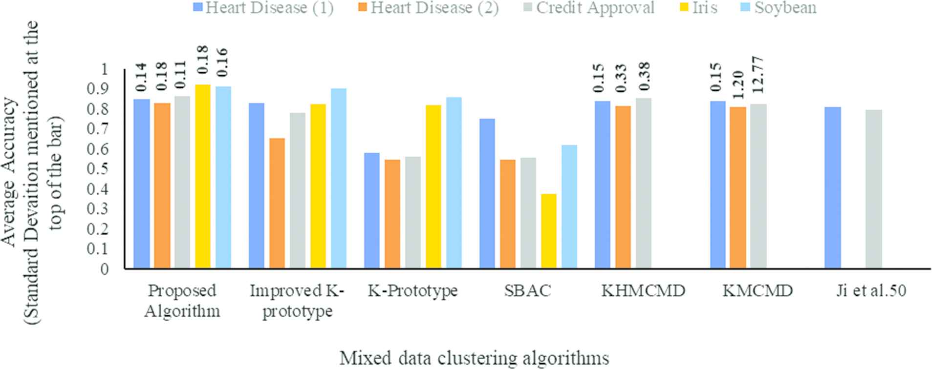
Comparison of clustering accuracy of proposed and existing clustering algorithms.
5.2. Application of the Proposed Clustering Algorithm to the Clustering of Postoperative Surgical Patients
Surgical patient clustering is defined as a process of arranging the patients in distinct groups based on their similarity of characteristics. These characteristics include age, gender, body mass index (BMI), American Society of Anesthesiologists (ASA) fitness grade, etc. For multi-specialty hospitals, where an enormous number of patients receive their surgical care, it is quite a challenging task to manage the surgical records efficiently. An efficiently managed surgical records help hospitals to improve patients care and monitoring to enhance the efficiency of resources within the hospital. In this paper, the surgical record management procedure (SRMP) of a multi-specialty hospital, India is examined, and the proposed algorithm is implemented on the hospital’s existing SRMP to cluster surgical records and enhance existing SRMP.
5.2.1. Dataset description
The historical postoperative surgical mixed dataset is obtained from Shri Mahant Indiresh Hospital, Dehradun, India. The description of the datasets is given in Table 5.
| Attribute | Type | Description |
|---|---|---|
| Age | Numeric | Patient’s age at the time of surgery |
| Gender | Categorical | Gender of patient |
| BMI | Numeric | Body mass index of patient |
| ASA fitness grade | Numeric | Patients physical status required by the anesthesiologist before surgery |
| Marital status | Categorical | Marital status of patients |
| Ethnicity | Categorical | Ethnicity of patient |
| Comorbidity | Numeric | Charlson comorbidity index |
| Type of surgery | Categorical | Classifies attempt of surgical procedure |
| Surgery duration | Numeric | Length of surgical procedure |
| Procedural code | Categorical | Primary procedure code |
| Diagnose code | Categorical | Primary diagnosis code |
| Surgery domain | Categorical | Classifies surgical procedure |
| Grade of surgery | Categorical | Classifies risk of surgical procedure to the life of the patient |
| Urgency of surgery | Categorical | Classify the schedule of a surgical patient |
| LOS | Numeric | Length of stay in hospital after surgery (in days) |
Postoperative surgical dataset characteristics.
5.2.2. Significance of active clusters selected by the proposed clustering algorithm
During each iteration of the algorithm, the significance of the obtained clusters are computed using two parameters: (1) frequency of the number of active clusters selected and (2) average accuracy.
5.2.3. Discussion
The experiments are carried out in 50 iterations, and the results obtained in the pair of 10-10 iterations are shown in Table 6. Table 6 demonstrates the frequency of selecting the active clusters and the average accuracy
| Iteration | No of Active Cluster Extraction |
|||||||
|---|---|---|---|---|---|---|---|---|
| 2 | 3 | 4 | 5 | 6 | 7 | 8 | ||
| 1-10 | 0.0 | 0.5 | 0.8 | 0.4 | 1.4 | 0.6 | 0.3 | |
| 0.0 | 0.51 (±0.63) | 0.62 (±0.42) | 0.47 (±0.36) | 0.77 (±0.18) | 0.59 (±0.48) | 0.44 (±0.44) | ||
| 11-20 | 0.4 | 0.5 | 0.9 | 0.6 | 0.6 | 0.8 | 0.2 | |
| 0.46 (±0..39) | 0.54 (±0.34) | 0.81 (±0.23) | 0.58 (±0.42) | 0.69 (±0.24) | 0.75 (±0.21) | 0.33 (±0.56) | ||
| 21-30 | 0.0 | 0.0 | 0.8 | 0.9 | 1.5 | 0.2 | 0.6 | |
| 0.0 | 0.0 | 0.68 (±0.35) | 0.78 (±0.21) | 0.86 (±0.14) | 0.37(±0.64) | 0.51(±0.60) | ||
| 31-40 | 0.3 | 0.0 | 0.9 | 1.0 | 1.2 | 0.0 | 0.6 | |
| 0.32 (±0.69) | 0.0 | 0.54 (±0.43) | 0.62 (±0.31) | 0.87 (±0.12) | 0.0 | 0.41 (±0.48) | ||
| 41-50 | 0.0 | 0.8 | 0.8 | 1.1 | 0.6 | 0.7 | − | |
| 0.0 | 0.46 (±0.36) | 0.53 (±0.62) | 0.82 (±0.21) | 0.39 (±0.46) | 0.48 (±0.54) | − | ||
The Numerical bold values represent the best results of Frequency (FQ), Average accuracy (AC), and Standard deviation (Sd) of the active clusters selected by the proposed clustering algorithm in each pair of 10-10 iterations.
Symbolic bold values FQ and AC represent Frequency and Average accuracy, respectively.
Frequency (
Finally, the active cluster with the maximum
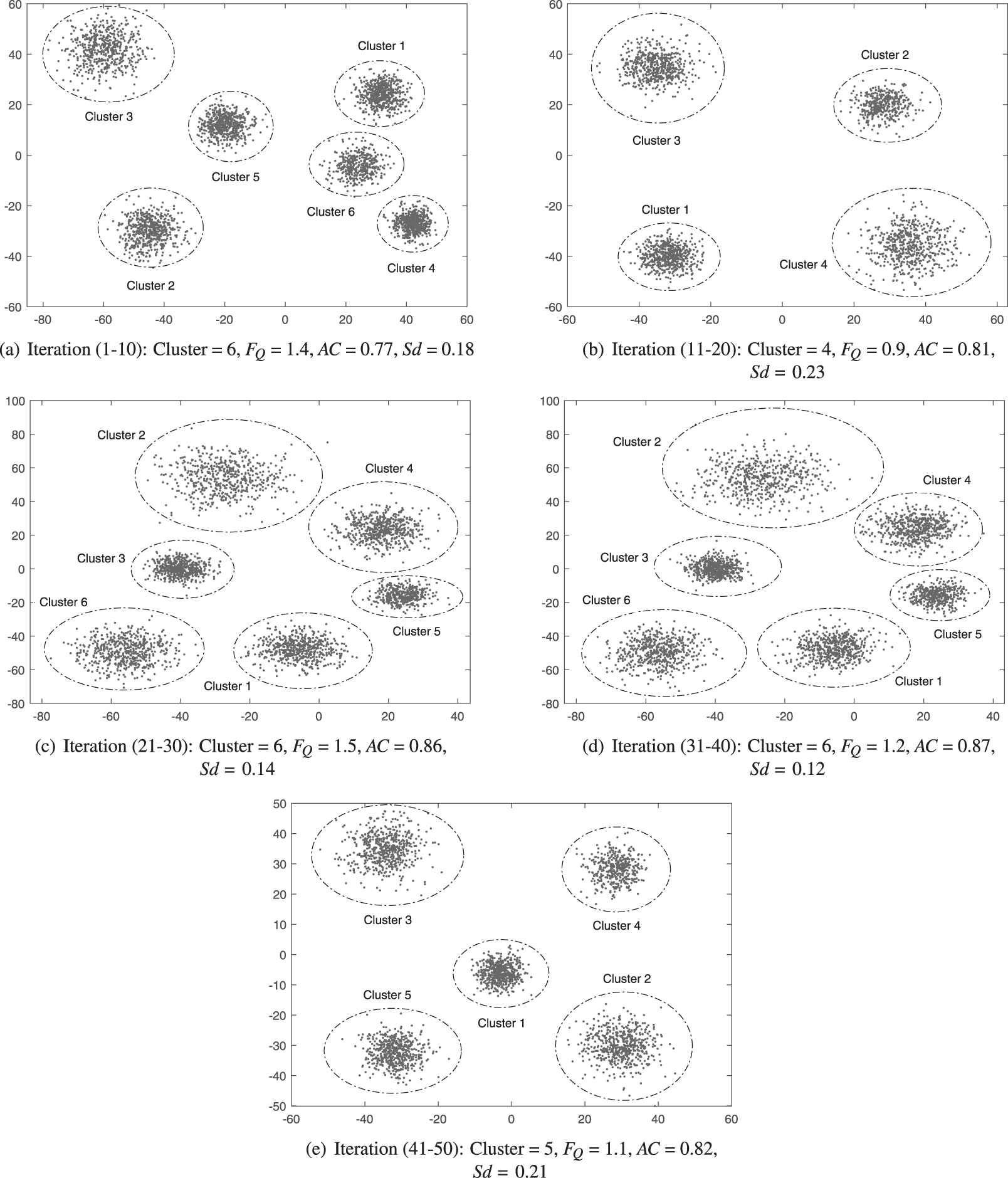
Cluster center selection frequency (FQ), average accuracy (AC) and standard deviation (Sd) for the postoperative surgical mixed dataset.
| Parameters | Value |
|---|---|
| No of active cluster obtained | |
| Frequency of active cluster selection ( |
1.2 |
| Average accuracy (AC) | 0.87 |
| Standard deviation ( |
Performance of the proposed clustering algorithm on the postoperative surgical dataset.
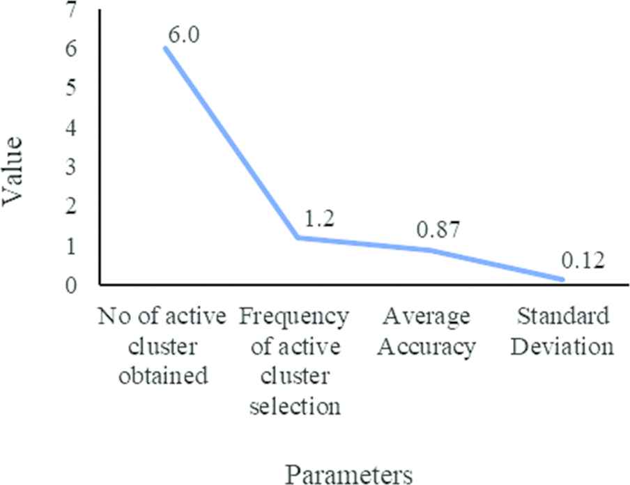
Cluster quality measures for the proposed algorithm for the surgical dataset.
5.3. Statistical Analysis of the Proposed Clustering Algorithm
Although results based on average accuracy (
| Dataset | Standard Error | t | 95% Confidence Interval | Two-tailed P-value | Significance |
|---|---|---|---|---|---|
| Heart Disease (1) | 1.000 | 10.0000 | −12.306 to −7.693 | 0.0001 | Highly significant |
| Heart Disease (2) | 1.811 | 13.0309 | −27.78 to −19.42 | 0.0001 | Highly significant |
| Credit approval | 1.00 | 5.0 | −7.306 to −2.693 | 0.0011 | Significant |
| Iris | 1.87 | 4.06 | −11.914 to −3.285 | 0.0036 | Significant |
| Soybean | 1.522 | 3.8335 | −9.28 to −2.39 | 0.0040 | Significant |
| Postoperative surgical dataset | 1.709 | 12.9450 | −9.0725 to −0.9916 | 0.000032 | Highly significant |
Unpaired t-test between the proposed and the second-best performing clustering algorithm for real-life datasets.
6. CONCLUSION AND FUTURE WORK
In this paper, AEFA is used to identify the number of clusters and cluster centers automatically. The proposed approach utilizes threshold setting and cut-off value to select and refine cluster centers. The assignment of data points to different clusters is made based on a distance measure, i.e., Euclidean distance for numeric attributes and the probability of co-occurrence of value for categorical attributes. The proposed approach requires no prior specification of the number of clusters. The proposed approach is compared with existing mixed data clustering algorithms based on robustness measures and statistical testing. The efficacy of the proposed approach is also validated by clustering real historical postoperative surgical patients dataset obtained from a multispecialty hospital. Experimental results evident that the proposed approach is not only able to automatically find the number of clusters, but also the clustering results are more robust and better than the existing clustering techniques. The clusters produced by the proposed approach are also compact and well separated. In the future, the proposed work can be enhanced in various directions: one direction can be solving the complex high dimensional clustering problems by hybridization of the proposed algorithm with other meta-heuristic approaches. Moreover, since the proposed algorithm automatically detects the optimum number of clusters, one can explore other heuristics to improve the optimal selection of clusters. The proposed algorithm can also be used in ensemble clustering.
CONFLICT OF INTEREST
The authors declare no conflict of interest.
AUTHORS' CONTRIBUTIONS
Conceptualization, Methodology, Formal analysis, Validation, Writing-Original Draft Preparation by Hemant Petwal and Supervision by Dr. Rinkle Rani. All authors read and approved the manuscript.
Funding Statement
This research received no external funding.
REFERENCES
Cite this article
TY  - JOUR
AU  - Hemant Petwal
AU  - Rinkle Rani
PY  - 2020
DA  - 2020/06/18
TI  - An Efficient Clustering Algorithm for Mixed Dataset of Postoperative Surgical Records
JO  - International Journal of Computational Intelligence Systems
SP  - 757
EP  - 770
VL  - 13
IS  - 1
SN  - 1875-6883
UR  - https://doi.org/10.2991/ijcis.d.200601.001
DO  - 10.2991/ijcis.d.200601.001
ID  - Petwal2020
ER  -