
Novel Cross-Entropy Based on Multi-attribute Group Decision-Making with Unknown Experts' Weights Under Interval-Valued Intuitionistic Fuzzy Environment
 , Yali Cheng, Qiong Mou, Sidong Xian
- DOI
- 10.2991/ijcis.d.200817.001How to use a DOI?
- Keywords
- Interval-valued intuitionistic fuzzy set; Experts' weights; Cross-entropy; Multi-attribute group decision-making
- Abstract
This paper studies the multi-attribute group decision-making problems with unknown experts' weights under interval-valued intuitionistic fuzzy environment. First, in order to provide more flexibilities for decision-makers in actual decision-making problems, a novel cross-entropy measure with parameter of interval-valued intuitionistic fuzzy set (IVIFS) based on J-divergence is proposed. The novel cross-entropy measure can obtain more flexible and practical optimal ranking results by adjusting the parameter. Then, by using the designed cross-entropy measure, two models are established to obtain experts' weights, which consider the influence of experts' experience and professional knowledge on experts' weights. Finally, two examples are provided to illustrate the effectiveness and applicability of optimizing the group decision-making approach.
- Copyright
- © 2020 The Authors. Published by Atlantis Press B.V.
- Open Access
- This is an open access article distributed under the CC BY-NC 4.0 license (http://creativecommons.org/licenses/by-nc/4.0/).
1. INTRODUCTION
Decision-making is generally considered a process in which human beings make choices among several alternatives [1]. In real life, due to the increasingly complex socioeconomic environment, it is impossible for a single decision-maker (DM) or expert to consider all relevant aspects of the decision-making problem without difficulty [2–6]. Therefore, many practical decisions are often made by multiple DMs or experts, which leads to abundant research concerning the topic of multi-attribute group decision-making (MAGDM) problems.
In MAGDM problems, DMs or experts should provide their preferences for alternative attributes to achieve a collective decision. Because of the uncertainty of the problem and the fuzziness of human thinking, it is difficult for DMs to evaluate alternatives with real numbers. There exist some hesitation and uncertainty inherent in DMs' judgments. Then, the intuitionistic fuzzy set (IFS) is defined in [7], which is just a strong tool to deal with hesitation and uncertainty [8]. Then the interval-valued intuitionistic fuzzy set (IVIFS) is proposed [9]. Since the membership and nonmembership of IVIF are described by intervals, IVIFS is better than IFS in representing fuzziness and uncertainty [10]. Since its appearance in the literature, the IVIFS and its extension theory has attracted increasing attention, many fuzzy MAGDM approaches have been presented [11–14].
In addition, how to obtain comprehensive weights of experts in MAGDM problems under IVIF environment is also the focus of many scholars. For example, a nonlinear optimization model is adopted [15], which minimizes the differences between individual and group opinions. Soon after, a method to derive experts' weights based on the distance between each matrix and the average matrix decision matrix is introduced [16]. Then, another method which depends on the difference between each matrix and the ideal group decision matrix is proposed [17]. However, the above methods for obtaining experts' weights do not consider the experience and expertise of experts. The experts' experience and the richness of professional knowledge determine the accuracy and reliability of experts' weights, and finally determine the feasibility of the sequencing scheme.
Since the entropy in the theory of information and developed the cross-entropy is introduced in [18], the fuzzy cross-entropy is defined to evaluate the relation between two sets or objects [19]. It is used to measure the divergence between two probability distributions or two random variables. After that, in [20], an effective application of the fuzzy cross-entropy MAGDM problems is showed. In [21], an integration of the cross-entropy under IF environments to solve MAGDM problems is proposed. A novel cross-entropy measure under IVIF environments to solve MAGDM problems is presented in [22]. An extended fuzzy cross-entropy measure of belief values based on a belief degree using available evidence is proposed to decision-making problems [23], and so on [24,25]. However, the above cross-entropy measures do not consider the psychology of DMs. The reliability and accuracy of decision results can be improved by describing decision psychology of DMs in decision-making methods [26].
Motivated by all mentioned above, in this paper, MAGDM problems with unknown experts' weights under IVIF environments are studied. The main contributions of this paper can be summarized as follows: (i) A novel cross-entropy measure with a free parameter of IVIFS is proposed based on J-divergence. Compared with the previous works [27,28], the proposed cross-entropy measure with parameter of IVIFS may provide more opportunities for DMs in actual decision-making, and it is more flexible and practical in order to obtain the optimal ranking results by adjusting the parameter. (ii) A new method in this paper is presented to obtain experts' weights, in which two programming models are constructed by considering the influence of experts' experience and professional knowledge on experts' weights.
The rest of the paper is organized as follows: Section 2 presents the preliminary concepts of IFS and IVIFS. In Section 3, the unknown expert weights are computed. Section 4 defines new cross-entropy measure under IVIF environments and studies its properties. In Section 6, an approach integrated previously proposed methods for MAGDM under IVIF environments is developed to select an optimal scheme. Two examples are given to illustrate the effectiveness and applicability of proposed methods in Section 6. Finally, Section 7 gives conclusion.
2. BASIC CONCEPTS OF IFS AND IVIFS
To describe the fuzzy nature of things more detailed and comprehensive, Atanassov initiated the concept of IFSs by extending FSs of Zadeh. This section is devoted to reviewing some basic notions of IFSs and IVIFSs.
Definition 1.
[7] Suppose that
In 1989, Atanassov and Gargov introduced IVIFS as a further generalization of IFS and gave the following definition.
Definition 2.
[9] Let
Similarly,
Another two important concepts for IVIFSs are deviation degree and cross-entropy measure which have been applied to many fields.
Definition 3.
[29] Deviation degree
Definition 4.
[20] For two IVIFNs
For any
For IVIFNs
Cross-entropy measure is often used to measure the discrimination information, in the light of Shannon's inequality in [30].
Definition 5.
[9] Supposing
In order to compare two IVIFNs
If
If
Definition 6.
[32] An
3. A MODEL-BASED METHOD TO DETERMINE THE WEIGHTS OF EXPERTS UNDER IVIF ENVIRONMENTS
Because the IVIFS can give a more reasonable mathematical skeleton to process inaccurate facts or imperfect information, in this section, we develop a comprehensive algorithm to integrate two models for obtaining appropriate experts' weights. Each expert's weight in our method is combined with two parts, the experience and the expertise of expert.
3.1. The Weighting Vector of Expert Determined by Experience Degree of Expert
Suppose that
By considering the experience of expert to compute the optimal expert's weighting vector, it can be formed as the following model:
To solve model (M-1), the Lagrange function is constructed as
By differentiating Eq. (1) with respect to
To solve above equations, we can get a simple and exact formula for determining the weights of experts as follows:
By standardizing
Therefore, we can get the expert's weighting vector
Further, from the viewpoint of similarity degree between pairwise individual decision matrices in [33] and [34], another optimization model based on the cross-entropy and the similarity measures for ensuring weights of experts can be constructed here.
3.2. The Weighting Vector of Expert Determined by Expertise of Expert
Let
Note that the closer the value of
Accordingly, for obtaining the expert's weighting vector, we concern similarity degree between individual decision matrices and expert evaluation matrices.
For differentiating Eq. (3) with respect to
By solving above equations, a simple and exact formula for determining the weights of experts can be get as follows:
By normalizing
Then we can get the weighting vector of expert that is
In practice, models (M-1) and (M-2) can be integrated for computing experts' weights in MAGDM under IVIF environment. The steps are summarized as follows:
Step 1. Calculate the fuzziness degree between individual decision matrix
Step 2. Compute the similarity degree between each individual decision matrix and matrices of expert evaluation, then get weighting vector of expert,
Step 3. Let
4. CROSS-ENTROPY MEASURE OF IVIFS
In this section, a new cross-entropy measure with parameter of IVIFS is constructed to support the proposed expert weight-determining method. We consider
By analogy information and based on the above, an information measure which is a divergence measure of two IVIFSs
Theorem 1.
The divergence measure
Proof:
Obviously,
Then, we have for all
Thereby, we can derive that
Remark 1.
If
Here
Remark 2.
Flexibility is an indispensable and important element in modern decision-making. Each individual is different, and DM tend to consider the problem from his own perspective. By adjusting parameter
5. INTEGRATED IVIF GROUP DECISION-MAKING APPROACH WITH UNKNOWN EXPERT WEIGHTS
Suppose that the information about the weighting vector of attribute is given in advance, that is,
Step 1. Get the collective IVIF decision matrices
Step 2. Obtain the weighting vector of expert
Step 3. Aggregate all the collective IVIF decision matrix
Step 4. From Definition 2.5, the values of the score function
Step 5. Obtain the priority of alternatives according to the above values of
6. ANALYSIS OF NUMERICAL EXAMPLES
In this section, some examples are illustrated to demonstrate the applicability of the proposed method. Meanwhile, the comparative analyses are also conducted to show the superiority of the proposed method.
6.1. Example 1
Suppose that
Assume that
From Eq. (5), we can obtain the cross-entropy between each pattern
| 0.0053 | 0.0058 | 0.0060 | |
| 0.0008 | 0.0009 | 0.0010 | |
| 0.0263 | 0.0253 | 0.0277 | |
| 0.0025 | 0.0031 | 0.0032 | |
| 0.0008 | 0.0009 | 0.0001 |
Cross-entropy between each pattern
By using the new cross-entropy measure Eq. (5), we can classify pattern
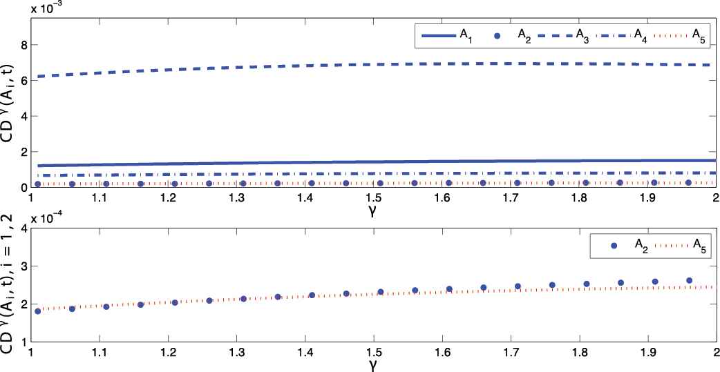
Values of in example 1.
Next, an example from [12], in which the weights of the attribute are known while the weights of the experts are unknown. Based on the aforementioned example, we show the method introduced in Section 4 is effective.
6.2. Example 2
Now, the information quality assessments of four social networks, Weibo (G1), QQ (G2), WeChat (G3), and Zhihu (G4) are taken into account. After a thorough investigation and evaluation, five attributes are constructed as
| ([0.45,0.70], [0.10,0.25]) | ([0.40,0.65], [0.20,0.30]) | ([0.60,0.80], [0.15,0.20]) | ([0.65,0.75], [0.10,0.20]) | |
| ([0.60,0.85], [0.05,0.10]) | ([0.45,0.65], [0.20,0.30]) | ([0.70,0.75], [0.15,0.25]) | ([0.35,0.60], [0.10,0.30]) | |
| ([0.65,0.80], [0.05,0.15]) | ([0.30,0.55], [0.35,0.45]) | ([0.35,0.50], [0.30,0.40]) | ([0.55,0.70], [0.15,0.25]) | |
| ([0.45,0.60], [0.25,0.35]) | ([0.55,0.75], [0.10,0.25]) | ([0.70,0.75], [0.10,0.20]) | ([0.40,0.70], [0.15,0.25]) | |
| ([0.35,0.60], [0.35,0.40]) | ([0.30,0.55], [0.20,0.40]) | ([0.60,0.65], [0.25,0.35]) | ([0.55,0.75], [0.05,0.20]) |
Decision matrix
| ([0.50,0.65],[0.05,0.30]) | ([0.45,0.60],[0.25,0.35]) | ([0.30,0.75],[0.05,0.20]) | ([0.55,0.70],[0.10,0.25]) | |
| ([0.65,0.80],[0.05,0.20]) | ([0.45,0.85],[0.05,0.10]) | ([0.55,0.70],[0.10,0.25]) | ([0.30,0.65],[0.15,0.30]) | |
| ([0.45,0.85],[0.10,0.15]) | ([0.40,0.60],[0.25,0.35]) | ([0.60,0.65],[0.20,0.30]) | ([0.55,0.70],[0.15,0.25]) | |
| ([0.70,0.80],[0.05,0.15]) | ([0.55,0.75],[0.10,0.20]) | ([0.60,0.65],[0.05,0.30]) | ([0.35,0.70],[0.15,0.25]) | |
| ([0.50,0.70],[0.10,0.25]) | ([0.55,0.60],[0.25,0.40]) | ([0.80,0.85],[0.05,0.10]) | ([0.20,0.65],[0.20,0.30]) |
Decision matrix
| ([0.50,0.55],[0.15,0.35]) | ([0.30,0.60],[0.20,0.30]) | ([0.45,0.75],[0.10,0.25]) | ([0.65,0.85],[0.05,0.15]) | |
| ([0.70,0.85],[0.05,0.10]) | ([0.55,0.60],[0.25,0.30]) | ([0.60,0.75],[0.15,0.20]) | ([0.20,0.50],[0.40,0.45]) | |
| ([0.55,0.65],[0.30,0.35]) | ([0.40,0.60],[0.10,0.30]) | ([0.70,0.75],[0.20,0.25]) | ([0.50,0.80],[0.05,0.20]) | |
| ([0.80,0.90],[0.05,0.10]) | ([0.60,0.80],[0.10,0.20]) | ([0.55,0.75],[0.15,0.20]) | ([0.20,0.45],[0.35,0.50]) | |
| ([0.65,0.85],[0.10,0.15]) | ([0.20,0.55],[0.30,0.40]) | ([0.50,0.60],[0.30,0.35]) | ([0.45,0.80],[0.05,0.20]) |
Decision matrix
The weighting vector of the attribute is known in advance and then the individual weighting vector of the expert is unknown. The following steps are given to select the optimal decision alternatives:
Step 1. Construct the aggregated overall individual IVIF decision matrices based on the opinions of experts.
Aggregate IVIF matrixes
| ([0.5393,0.7416],[0.1041,0.2083]) | ([0.5959,0.7821],[0.0643,0.1881]) | ([0.6888,0.8214],[0.0921,0.1612]) | |
| ([0.4321,0.6573],[0.1770,0.3207]) | ([0. 4942,0.7109],[0.1398,0.2397]) | ([0.4656,0.6763],[0.1542,0.2750]) | |
| ([0.6197,0.7059],[0.1634,0.2614]) | ([0.6094,0.7173],[0.0738,0.2291]) | ([0.5741,0.7294],[0.1691,0.2364]) | |
| ([0.4896,0.7016],[0.1103,0.2412]) | ([0.3954,0.6839],[0.1493,0.2660]) | ([0.3853,0.6842],[0.1367,0.3004]) |
A overall individual interval-valued intuitionistic fuzzy set (IVIF) decision matrix
Step 2. Determine weighting vector of expert.
By utilizing Eqs. (2) and (4), the weighting vector of expert can be obtained as follows:
Step 3. Obtain the overall group decision matrix.
Combined with the IVIFWA operator and Eq. (6), the overall individual decision matrix
| Alternative | |
|---|---|
| ([0.6114,0.7835],[0.0846,0.1853]) | |
| ([0.4650,0.6828],[0.1560,0.2759]) | |
| ([0.6020,0.7175],[0.1251,0.2418]) | |
| ([0.4256,0.6900],[0.1312,0.2676]) |
The overall group decision matrix
Step 4. By Definition 2.3, the scores of values in
Step 5. Rank the alternatives.
On the base of the scores of
Comparative analysis: To further shown the superiority of our approach in comparison with other group decision-making methods, for example, in [10,23,38,39], some simulation results are depicted in Table 7.
| Methods | Ranking Results |
|---|---|
| Method in this paper | |
| Method in [23] | |
| Method in [10] | |
| Method in [38] | |
| Method in [39] |
Ranking results of different methods for Example 2.
From Table 7, we can get the alternative ranking result given by the method in [23,38] is the same with that given by our method. And the ranking results obtained by the proposed method in this paper are different from those obtained by methods [10,39]. On the basis of the above simulation results, we can find that the proposed method in this paper has some advantages over methods in [10,23,38,39].
(1) Each expert has the same weight in [39] and the weight to each expert is assigned in advance [10]. Both two methods neglected the determination of experts' weights. To overcome the shortcoming, experts' weights for each attribute are derived in [23,38] by using the similarity degree and proximity degree. But they do not consider the influence of experts' experience and professional knowledge on expert weights. By contrast, a new method in this paper is presented to obtain experts' weights, in which two programming models are constructed by considering the influence of experts' experience and professional knowledge on experts' weights. Moreover, the proposed method can provide more opportunities for DMs in actual decision-making by proposing a novel cross-entropy with parameter, which is comprehensive and flexible.
(2) The alternatives ranking method in [39] is to calculate the distances between IVIF positive ideal solution and schemes, but this method is not robust for different IVIF positive ideal solutions. The alternatives ranking method in [38] is directly transformed the IVIF matrix into an interval matrix, which could result in information loss. The ranking method in [10] is the same as the ranking method in [40]. And the ranking order of alternatives is generated according to an order relation of IVIFVs in [23]. However, the above ranking methods cannot provide more opportunities for DMs in actual decision-making, so these methods also cannot be applied to different DMs and different decision-making environments. By contrast, the method in this paper can be applied to different DMs and different decision-making environments by adjusting the parameters. Furthermore, it has some desirable properties and advantages over existing ones.
Discussion of the influence of parameters: It is necessary to discuss whether and how the ranking results change when the values of these parameters
| Methods | Ranking Results |
|---|---|
Computation results with different values of parameters
It can be seen from Table 8 that the ranking order of alternatives is not the same for different decision principles of DMs when the value of parameters
7. CONCLUSION
In this paper, MAGDM problems with unknown experts' weights under IVIF are investigated by fully considering the experts' experience and professional knowledge. Then, a novel cross-entropy measure with parameter of IVIFS based on J-divergence is proposed to handle the MAGDM problems. Next, in order to further show the effectiveness of the proposed method, comparative case studies have been carried out. Compared with the existing representative cross-entropy measures [22,23], the proposed cross-entropy has better discriminating ability. Furthermore, we can further study and extend it to other practical fuzzy decision-making environments, such as the fuzzy group decision-making support system under the interactive intelligent decision framework of green suppliers.
CONFLICT OF INTEREST
The authors declared that they have no conflicts of interest to this work.
AUTHORS' CONTRIBUTIONS
All authors contributed to the work. All authors read and approved the final manuscript.
ACKNOWLEDGMENTS
This work was supported by the National Natural Science Foundation of China (Grant Nos. 11671001 and 61472056), the Technological Research Program of Chongqing Municipal Education Commission of China (Grant no. KJ1600425), and the Science and Technology Research Project of Chongqing Municipal Education Commission (Grant No. KJQN201800624).
APPENDIX
A proof of Theorem 4.1
The
Obviously,
Though the above discussion,
From the Theorem 1 in [41], we can obtain
Thereby,
Therefore,
REFERENCES
Cite this article
TY  - JOUR
AU  - Yonghong Li
AU  - Yali Cheng
AU  - Qiong Mou
AU  - Sidong Xian
PY  - 2020
DA  - 2020/08/29
TI  - Novel Cross-Entropy Based on Multi-attribute Group Decision-Making with Unknown Experts' Weights Under Interval-Valued Intuitionistic Fuzzy Environment
JO  - International Journal of Computational Intelligence Systems
SP  - 1295
EP  - 1304
VL  - 13
IS  - 1
SN  - 1875-6883
UR  - https://doi.org/10.2991/ijcis.d.200817.001
DO  - 10.2991/ijcis.d.200817.001
ID  - Li2020
ER  -