
A Simulation Method of Specific Fish-Eye Imaging System Based on Image Postprocessing
 , Ying Wang, Jialun Liu
- DOI
- 10.2991/ijcis.d.201126.001How to use a DOI?
- Keywords
- Sensor simulation; Intelligent vehicle system; Fish-eye camera; Camera calibration; Stereographic projection model
- Abstract
In order to enable the implementation of the computer vision-based perception techniques in the physical-based simulation environment, visual sensors need to be simulated physically. Among others, fish-eye cameras are commonly used visual sensors to provide an omni-directional field of view. The existing methods cannot simulate the output of a specific real fish-eye imaging system. In this paper, we present a postprocessing fish-eye imaging system simulation method. According to the stereographic projection model, a mapping is established between the ideal fish-eye image and a cube-map rendered by the graphic engine. The distortion of the real camera is measured and added to the ideal image, in order to simulate the output of a specific camera. Experimental result shows that our simulation method can give output close enough to the image captured by a specific fish-eye camera. The practicality of our method is validated in an actual application of vehicle omniview system.
- Copyright
- © 2021 The Authors. Published by Atlantis Press B.V.
- Open Access
- This is an open access article distributed under the CC BY-NC 4.0 license (http://creativecommons.org/licenses/by-nc/4.0/).
1. INTRODUCTION
Over the years, physical-based simulation tools are widely used in many industrial fields, such as intelligent vehicle [1] and robotics [2]. In the early stages of development of intelligent vehicle systems, making prototype experiments in a virtual environment can help reducing the experiment cost, protecting the safety of persons and devices, and avoiding the legal and moral risk. There are several intelligent vehicle-dedicated simulation platforms on the market. Pro-SiVIC of CIVITEC is a sensor simulator. It can simulate various complex scenarios like roundabouts, multiple vehicles and pedestrians, and different weather conditions. Some applications [3] use Pro-SiVIC simulator to test cooperative algorithms on intelligent vehicles. CarSim [4–6] of the Mechanical Simulation Company, providing dynamics vehicle models, is designed to validate driving assistance algorithms. PreScan [7] of Tass International is also a simulator that is specialized on sensor modeling. It has a full-spectrum camera simulation for reliable virtual development and validation of automated driving applications. In the industrial production, off-line programming of the industrial robots in simulation software can reduce the frequency of stoppage of the production line, so as to reduce the impact on production efficiency. While almost every robot manufacturer offers a brand-specific simulation tool, there are also many third-party simulators like CoppeliaSim [8], Robotmaster [9], Delfoi [10], etc. In the abovementioned intelligent or automatic systems, various sensors are mounted to provide information about the surrounding situations. Among others, visual sensors are the most commonly used ones [11]. The functions of these sensors need to be reproduced physically in the simulation tools.
Nowadays, in many applications such as intelligent surveillance [12,13] and autonomous navigation [14,15], an omni-directional field of view (FOV) is often required in order to see more in one shot. Compared with other omni-directional imaging systems, such as multi-camera devices [16,17] and catadioptric cameras [18,19], fish-eye cameras, which combine fish-eye lenses and conventional cameras, are cheaper, smaller, and easier to set up, and thus are becoming increasingly popular in the computer vision community.
There are few simulation methods dedicated to the fish-eye cameras. The Pro-SiVIC platform chooses two techniques to simulate omni-directional cameras. The first one generates fish-eye images by merging 6 images rendered by the OpenGL library, which takes no account of the imaging geometry of real cameras. The second one uses a mesh to form the desired shapes and reflect the environment on it. It also cannot be used to generate the output of a specific fish-eye camera. Ref. [20] presented a three-dimensional simulation method for fish-eye lens distortion in a vehicle rear-view camera. This method can only generate the image of straight lines, and needs the field number of the target fish-eye lens, which is not always available. In summary, for the following reasons, it is necessary to propose a new simulation method for fish-eye cameras:
Physical-based simulation technology is widely used in the field of intelligent system;
Fish-eye camera is widely used in computer vision technology, the latter is one of the main technologies in intelligent systems;
So, it is necessary to provide a method to simulate a specific fish-eye camera in the physical-based simulation environment;
However, there are few existing methods to simulate the output of a specific fish-eye camera.
In this paper, we proposed a postprocessing method to simulate the output of a specific fish-eye imaging system. The graphic engine is used to generate a cube-map centered on the principal point of the fish-eye camera, and then the relationship between the pixels on the simulated fish-eye image and the cube-map is established according to the fish-eye imaging model, i.e., the stereographic projection model. Then the simulated fish-eye image is generated. The essence of this method is to transform the image pre-generated by the engine, which is called “postprocessing method.” To make the simulated image closer to the real output of a specific device, the deviation from the ideal projection model to the imaging geometry of a real camera is estimated quantificationally and applied to the fish-eye image. Experimental result shows that our simulation method can give output close enough to the image captured by a specific fish-eye camera. The practicality of our method is validated in an actual application of vehicle omniview system.
This paper is organized as follows: Section 2 introduces the projection models used to describe a fish-eye imaging system. The proposed simulation method is detailed in Section 3. After providing experimental results and validations in Section 4, Section 5 concludes the paper.
2. PRELIMINARIES
2.1. Projection Models
A projection model is a mapping from the 3D object point
In addition to the projection model, imaging system design usually involves many other considerations, e.g., size, cost, and uniform illumination. Assembly defects are also introduced during camera manufacture. These will make the actual output of cameras deviates from the ideal projection model to varying degrees. This deviation is often treated as distortion. In classical camera calibration methods, the most commonly used distortion model is the Brown–Conrady polynomial model [21]:
Here,
The FOV of a pinhole camera is restricted by the size of the sensor. To take the entire scene of a
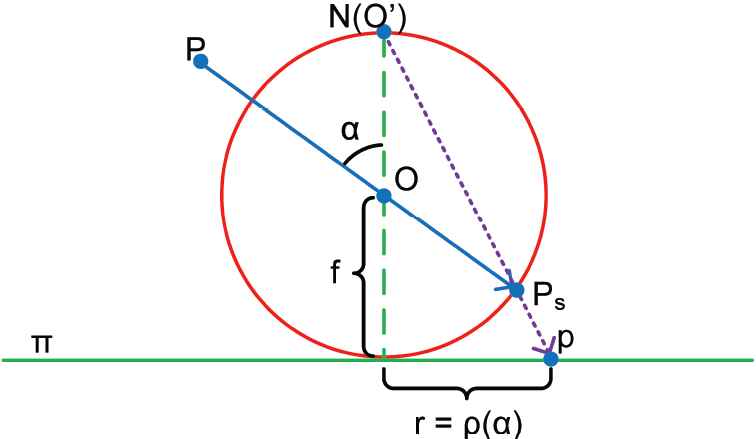
Two-stage procedure for describing a projection model. A 3D point is first projected onto the viewing sphere, followed by another perspective projection from some point on the optical axis onto the image plane.
First, a 3D point
Note that the perspective projection can also be described by this procedure. In Ref. [23], the author prefers to stereographic projection rather than other alternative ones because it can represent a wider FOV while preserving a suitable range of shape properties of the projected objects, including the circularity, the local symmetry, the shape of small regions, and the angle at which two curves intersect. These properties are very useful in applications such as intelligent surveillance and automatic navigation. Thus, in this paper, the stereographic projection model is chosen for our estimation method. It is exactly the model shown in Figure 1.
2.2. Geometric Invariants Under Stereographic Projection
Simple geometric targets, such as straight lines or spheres, are often utilized in the distortion estimation methods because the shape of the images of these targets is known under a certain projection model. For stereographic projection, this is shown in Figure 2.
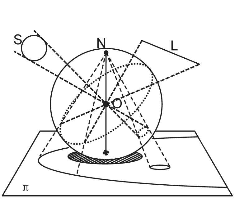
Images of a line and a sphere under the stereographic projection. The projection of a space line on the viewing sphere, as well as the projection of a sphere (dotted line), is a circle. Circles on the viewing sphere maintain their shape when projected onto the image plane from the northern pole of the viewing sphere (solid line on the image plane).
When projected onto the viewing sphere from its center
We set
Notice that both (4) and (5) are the general equations of a circle. So the conclusion is that the image of a space line section under the stereographic projection is a circular arc (a portion of a circle), and the image of a sphere is a circle. These are the main geometric invariants used in our estimation method.
3. SIMULATION METHOD DETAILS
In this section, we propose a fish-eye image generation method based on the engine-rendered image postprocessing. First, an ideal fish-eye image is generated. To get the value of a particular pixel in the output image, the corresponding incident ray is back-traced into the virtual environment according to the projection model. To simplify the implementation, a cube-map centering at the center of the viewing sphere is rendered with the help of a 3D graphic engine. Then, the distortion parameters of the target camera are estimated and used to distort the ideal image in order to connect the simulation to the specific imaging system.
3.1. Generate the Ideal Fish-Eye Image
The common method to generate images of a virtual scene is backward ray-tracing. For fish-eye camera simulation, it is the inverse procedure of the projection model described in last section. For a given 2D point
From the stereographic projection function given in (3), the incident angle
Actually, in order to achieve a more realistic rendering effect, the tracing may not stop at
We define 6 identical pinhole cameras in the virtual scene, all positioned at the center of the viewing sphere. The cameras are arranged orthogonally. If the orientation of the fish-eye camera is (0, 0, 1), then the orientations of the 6 pinhole cameras are (0, 0, 1), (0, 0, −1), (0, 1, 0), (0, −1, 0), (1, 0, 0), (−1, 0, 0), respectively. The cameras all have an FOV of 90 degrees in both horizontal and vertical directions. The deployment of the cameras is shown in Figure 3.
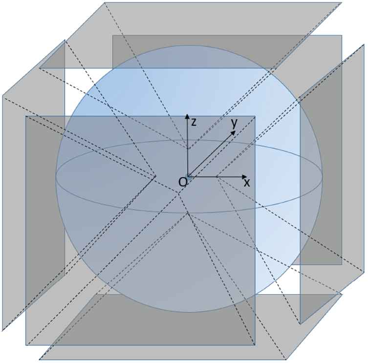
The viewing sphere and the deployment of the six pinhole cameras. The cameras are moved from their original position (i.e., the center of the viewing sphere) along the axis to make the figure clearer.
In this way, the images rendered through these six cameras form a cube-map. In our simulation, only five cameras are sufficient. The camera looking backward is omitted because we just need an FOV of 180 degrees in front of our fish-eye camera.
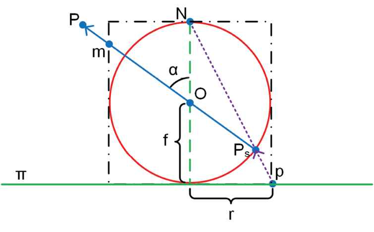
Mapping from the fish-eye image plane to the five orthogonal cameras. The incident light ray is back-traced and hits one of the faces of the cube-map at a point.
This creates a mapping between the simulated fish-eye camera and the five cameras. This mapping doesn't change from frame to frame in real-time rendering, thus can be stored in a mapping table. Each camera is assigned an ID, and for a pixel in the output image, its corresponding entry in the lookup table is like
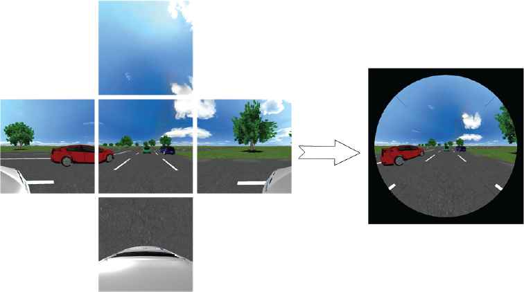
The rendered outputs of the five cameras and the simulated ideal fish-eye image.
3.2. Image Distortion
Figure 6(a) shows the ideal image of several spheres generated by the method described in last section. According to the property of the stereographic projection, the image of a sphere is a circle. However, it is not the case in a real fish-eye image as shown in Figure 6(b).
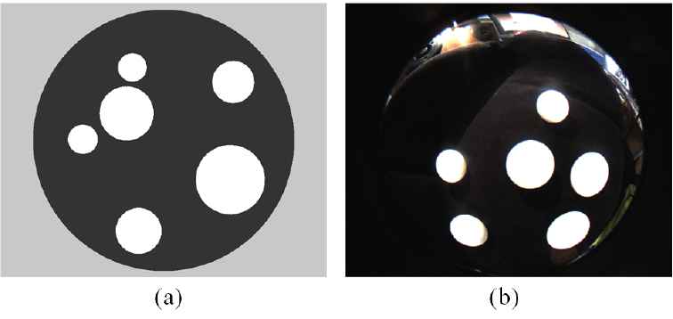
(a) The simulated ideal fish-eye image of several spheres. (b) Image of spheres captured by a real fish-eye camera.
In this section, we detail our distortion estimation method. The estimation of the distortion center and the distortion coefficients are performed in a hierarchically iterative manner because it has been shown that including the distortion center in the nonlinear optimization may make the system unstable with the presence of noise [21]. In the outer loop, feature points extracted from images of parallel lines are undistorted with the latest estimated distortion parameters and then used to update the distortion center. If the new center is close enough to the current one, the algorithm terminates. Otherwise, in the inner loop, with the latest distortion center, a genetic algorithm (GA) module is adopted to optimize the distortion coefficients based on the geometric invariants discussed in Section 2.2.
3.2.1. Estimation of the distortion center
We estimate the distortion center with the help of the vanishing points. A vanishing point is the intersection of a group of parallel straight lines under the stereographic projection model. A straight line in space can be given as a point direction form equation as
Let
From the perspective and stereographic projection functions in (3), the radial distance of the corresponding point
Rearranging gives
The projection of a given 3D point under different projection models always moves along the radial direction. Therefore, the projected 2D points are related by their radial distance:
Inserting (10) and (12) into (13) gives
The limit of (14) as
If we consider the two points as two vectors from the distortion center, examining the angle
Extract points. An edge detection algorithm such as Sobel or Canny is used to extract the points on the image of lines. As shown in Figure 7(a), the extracted points are grouped into several sets:
where for eachUndistort the points and do circle fitting.
Initialize the vanishing points. An initial guess is required for the optimization. The intersections of every two circles in
whereOptimize the vanishing points. The initial positions of
Estimate the distortion center. Several other pairs of vanishing points are determined from other pictures of the parallel lines in the same way. The lines joining each pair of vanishing points intersect with each other, and the centroid of the intersections is located as the distortion center, as shown in Figure 7(d).
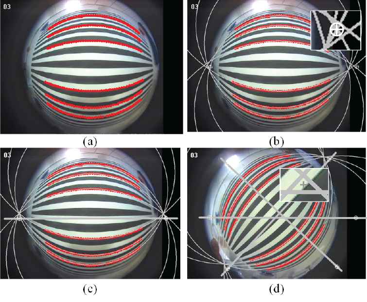
Estimation of the distortion center: (a) Points on the images of lines are extracted and grouped into several sets. (b) The fitting circles have many pairs of intersections, and the one with the lowest score is chosen as the initial position of the vanishing points. (c) The initial points are optimized and then linked. (d) At least three pairs of vanishing points need to be estimated to determine the distortion center.
3.2.2. Estimation of the distortion coefficients
In this subsection, the geometric invariants discussed in Section 2.2 are used to estimate the distortion coefficients of the fish-eye cameras. We need to define an object function by which, when minimized, the distortion parameters are optimized to put the points extracted from the image of the geometric targets back onto given shapes. Our object function is defined via the images of spheres as well as straight lines. As we will show later in Section 4, spheres are more appropriate to serve as the geometric target for the distortion estimation of fish-eye cameras, especially with the presence of measurement noise.
The first two steps are similar to the ones described in last subsection. Pictures of the target objects (lines in space or spheres) are captured, and edge points
Measurement noise in the extracted points will be amplified nonlinearly due to the distortion if the objective function is defined in the space of the undistorted points [24]. Thus, in this paper, we define the object function in the space of distorted image points to ensure the robustness of the estimation method with the presence of noise. As shown in Figure 8,
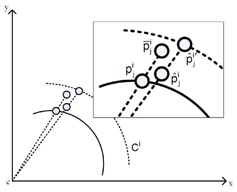
Setup for determining objective function.
The GA is used here to minimize (19). A simple GA using single-point crossover and single-point mutation is sufficient for our problem. Any other nonlinear optimization algorithm could also be used here. Once the distortion parameters are determined, the distorted position of the pixels in the ideal image can be found, and the mapping relationships between the output image and the cube-map recorded in the mapping table need to be adjusted accordingly.
4. EXPERIMENTAL RESULTS AND DISCUSSION
In this section, three sets of experimental results are presented to show the robustness of our estimation method. In the first experiment, all image points are artificially generated, thus the distortion-free position of the image points is known. In the second experiment, a 3D engine is employed to construct a virtual scene containing the geometric targets. The method is applied to the images rendered by the 3D engine. The procedures that may introduce noise, including image acquisition and point extraction, are involved. This makes the experiment closer to the real situation. We then apply our method to the real images, and give a quantitative evaluation of our simulation method. Finally, an actual application of vehicle omniview system is implemented to show the practicality of our method.
The GA module searches the distortion coefficients in the intervals
4.1. Experiment on Fully Synthetic Points
In this experiment, we show how the number of the target objects affects the estimation result with the presence of noise of different levels. The effectiveness of lines and spheres as the target is also compared. A fish-eye camera using an 800*800 CCD sensor is considered. With a focal length of 160 pixels, the whole FOV of
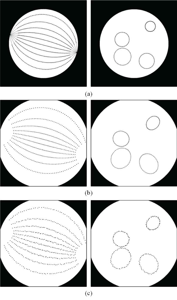
Illustration of the experiment using fully synthetic data. (a) Points on the ideal image. (b) Points in (a) are distorted. (c) Distorted points are contaminated by Gaussian random noise.
Next,
In a single run of the estimation, a group of three
We vary the noise level
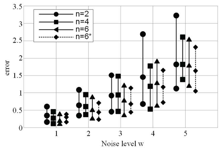
The inter-quartile range (IQR) of is fixed at 0.
Although becoming larger with the increasing noise level,
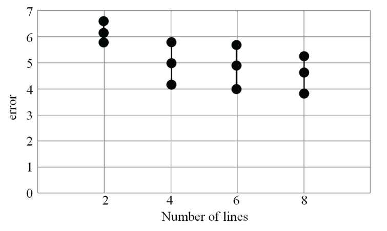
On the other hand, when a group of lines is used as the target, the result is not so good, as show in Figure 11. Even if the number of the lines increases, the improvement of the result is limited. The main reason for this is that the image of a space line under stereographic projection is only a portion of a circle, and circle fitting with points lying on a portion of a circle is an ill-conditioned problem. When a circle is fitted to these points, owing to the stronger fitting capacity of quadratics and the lack of geometric constraints, the objective function (19) has a great chance of reaching the minimum even if the undistorted points are very far from the ground truth. This will cause the iteration to converge to the wrong parameters. However, the image of a sphere is itself a complete circle; thus, the problem described above will not exist when spheres are used.
The inter-quartile range (IQR) of is set to 1.
4.2. Experiment on Simulated Images
The complete process of the method is carried out in this experiment, including the extraction of the image points. The experimental setup is the same as that described in Section 4.1 except that the ground truth of the points doesn't exist. The parameters of the distortion are still known. Therefore, in this section, we directly examine the estimated parameters. To obtain the simulated images, two virtual scenes are created by the OGRE engine, as shown in Figure 12(a) and 12(b).
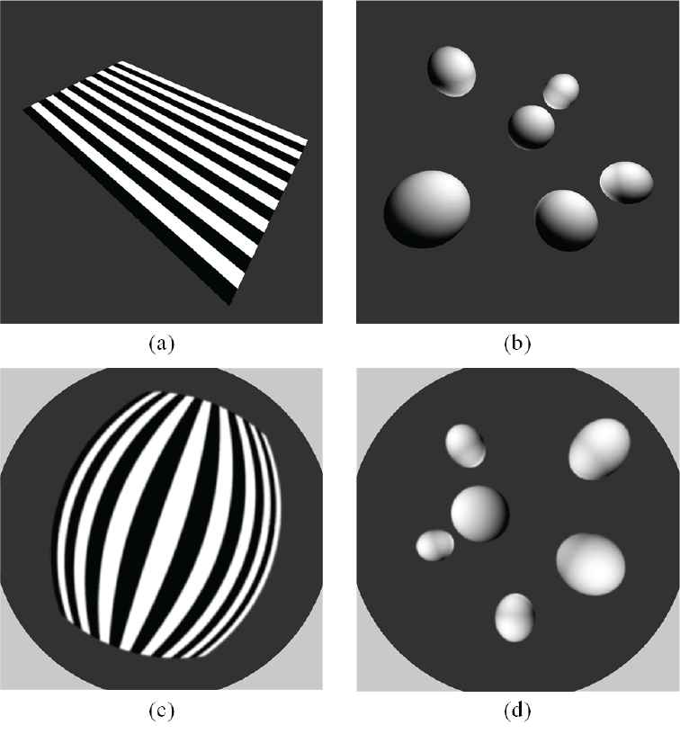
(a) and (b) Scenes containing a plane textured by black-and-white stripes and some spheres, respectively. (c) and (d) Distorted fish-eye images of (a) and (b), rendered by the modified OGRE engine.
Scene 1 contains a plane target textured by some stripes to provide parallel lines. Scene 2 contains several identical spheres placed at random positions. We don't care about the interval between the lines and the size of the spheres. We have modified the engine to render blurry images. A Gaussian Blur with a radius of 2 pixels is applied here, and the coefficients
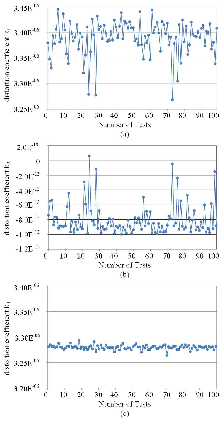
(a) and (b) Results of 100 runs of our method with the same test set. Both is fixed at 0.
The result shows that when both of the coefficients are estimated, the value of
4.3. Experiment on Real Images
In this subsection, we give a quantitative evaluation of our simulation method. The error between the relative distortion of the real and the simulated image is measured.
The device used in the experiment is an inexpensive fish-eye camera. The size of its sensor is 704*576 in pixels. The distortion parameters are estimated from the pictures of the targets, as shown in Figure 14.
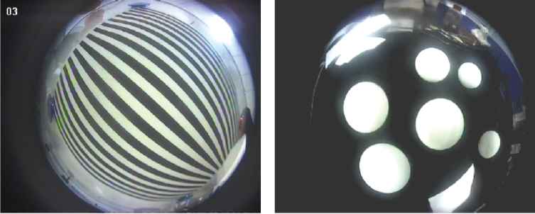
Images captured by a real fish-eye camera used to estimate the distortion.
The estimation result is
A chessboard pattern is captured with the target device, and the corresponding simulated image is given, as shown in Figure 15.
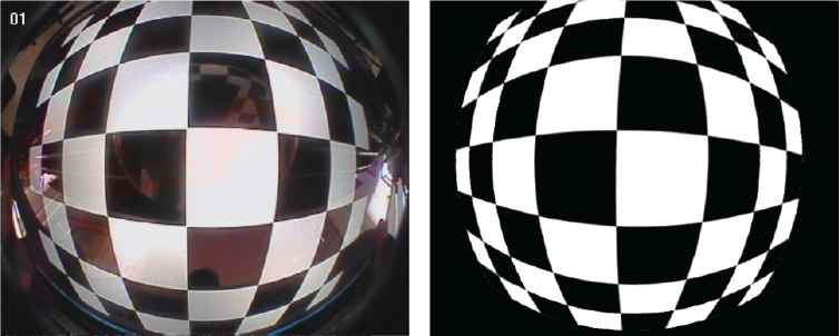
An image of a chessboard pattern captured by the real fish-eye camera and the corresponding simulated image.
Corners are extracted from both of the images. The ratio between the radial distance of the corners in the observed image and their distortion-free positions is a relative measure of distortion. The similarity between the real and the simulated image can then be determined by comparing this ratio, as shown in Figure 16.
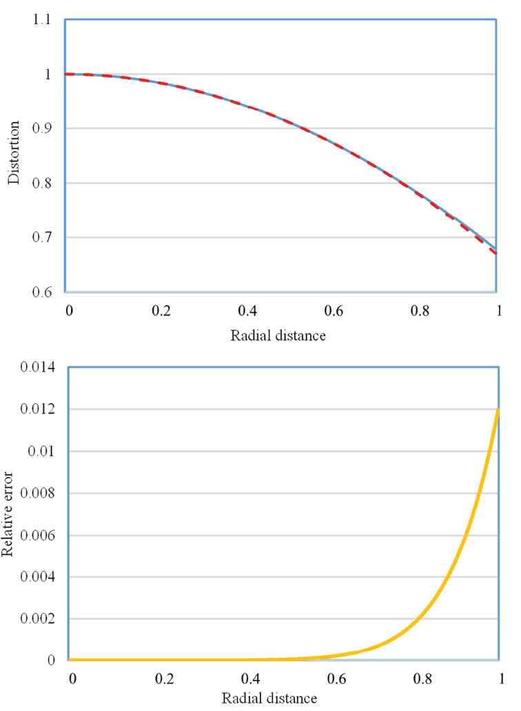
The ratio between the ideal and distorted position of the corners in the real and simulated image and the relative error calculated between the two images.
For points near the image center (radial distance smaller than 60%), the relative error is very small. The error increases with the radial distance, which could have been expected due to the limited number of terms used in the distortion polynomial. At the edge of the images, the error between the real and the simulated images is about 1.2%. This is a good enough result.
4.4. Validation of Practicality
In this subsection, the practicality of our method is validated through an actual application of vehicle omniview system. In a common vehicle omniview system, there are often four fish-eye cameras mounted: one in the front of the vehicle, one in the back of the vehicle, one in the left outside mirror, and one in the right outside mirror. These four simulated fish-eye images are shown in Figure 17(a). The imaging system simulated above is used here. The ground is textured with chessboard pattern to clarify the result. The inverse perspective transformation is adopted to transform the image parts containing the ground into top views according to the parameters of the cameras. The top views are then fused into one single omniview image, as shown in Figure 17(b).
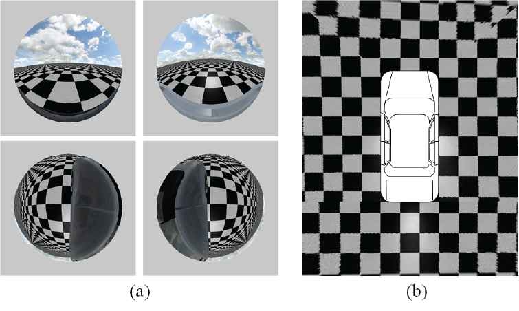
(a) The simulated images from the four fish-eye cameras mounted on the vehicle. (b) The omniview image generated from the images in (a).
As we can see, compared with the sides of the vehicle, the top views of the ground in front and rear of the vehicle are more blurred and mismatched. The main reason of this is the mounting angle of the cameras. Both of the side cameras look straight downward, while the cameras on both ends of the vehicle raise their line of sight in order to avoid being occlude by the bumpers. The image parts of ground in these images are closer to the edge, where the distortion is more severe. The quality of the top view transformed from these images is poor. To solve this, we can modify the algorithm, change the camera mounting position, or even consider other cameras. In this way, problems can be found before the assembling of the actual system and the cost is saved.
5. CONCLUSION
In this paper, we presented a postprocessing method to simulate the output image of fish-eye cameras. The proposed method establishes a pixel-wise mapping between the simulated image and the cube-map rendered by a graphic engine, according to the stereographic projection model. For a given pixel position in the simulated image, a direction vector starting from the origin is determined. Its pixel value can be obtained from the pixel pointed by this vector in one of the prerendered images. The output of this step is an ideal fish-eye image. It has nothing to do with any specific camera. After the mapping is established, the distortion parameters of the camera is taken into account. We proposed a robust estimation method of the distortion parameters of the fish-eye imaging system. It outputs the position of the distortion center on the image plane of the camera, and the coefficients of a polynomial describing the radial distortion in the fish-eye image. The method was tested on synthetic, simulated, and real images. The experimental results showed that our method can yield accurate parameters even in the presence of noise. The estimated distortion parameters are then used to adjust the mapping relationship. A major contribution of this work is the camera-specific simulation that optimizes the efficiency of the algorithm development and the cost of the selection and preinstallation of the equipment in intelligent perception systems using fish-eye cameras. Also, the proposed simulation method is easy to implement and less expensive than existing commercial simulators.
DATA AVAILABILITY STATEMENT
All data used to support the findings of this study are included within the article.
CONFLICTS OF INTEREST
The authors declare they have no conflicts of interest.
AUTHORS' CONTRIBUTIONS
All authors contributed to the design and implementation of the research, to the analysis of the results, and to the writing of the manuscript. All authors read and approved the final manuscript.
Funding Statement
The funding sources have made a financial contribution to the research and the preparation of the article. They had no involvement in the work beyond providing a financial contribution.
ACKNOWLEDGMENTS
This work was supported by the National Natural Science Foundation of China (NSFC) under Grant No. 51805203, and by Jilin Scientific and Technological Development Program under Grant No. 20190201023JC, and by the Development and Reform Commission of Jilin Province under Grant No. 2019C054-2.
REFERENCES
Cite this article
TY  - JOUR
AU  - Wenhui Li
AU  - You Qu
AU  - Ying Wang
AU  - Jialun Liu
PY  - 2020
DA  - 2020/12/02
TI  - A Simulation Method of Specific Fish-Eye Imaging System Based on Image Postprocessing
JO  - International Journal of Computational Intelligence Systems
SP  - 238
EP  - 247
VL  - 14
IS  - 1
SN  - 1875-6883
UR  - https://doi.org/10.2991/ijcis.d.201126.001
DO  - 10.2991/ijcis.d.201126.001
ID  - Li2020
ER  -