
Parallel DNA Algorithms of Generalized Traveling Salesman Problem-Based Bioinspired Computing Model
 , Tunhua Wu2, *
- DOI
- 10.2991/ijcis.d.201127.001How to use a DOI?
- Keywords
- DNA computing; Adleman–Lipton model; Generalized traveling salesman problem; NP-hard problem
- Abstract
Generalized traveling salesman problem (GTSP) is a classical combinatorial optimization problem, in which the optimization goal is the minimum route combination. Since the GTSP is a more complex problem than the traveling salesman problem (TSP), the GTSP can be considered an extension of the TSP. At present, compared with TSP, GTSP has been widely used in practice. In GTSP,
- Copyright
- © 2021 The Authors. Published by Atlantis Press B.V.
- Open Access
- This is an open access article distributed under the CC BY-NC 4.0 license (http://creativecommons.org/licenses/by-nc/4.0/).
1. INTRODUCTION
It is well known that the generalized traveling salesman problem (GTSP) is a generalization of the traveling salesman problem (TSP), and therefore is a nondeterministic polynomial (NP) problem. TSP is a commodity salesman from a city to several cities to sell commodities, and he needs to back home after all. The question is how he should arrange the route to minimize the cost of the tour. In the language of graph theory, given a connected graph
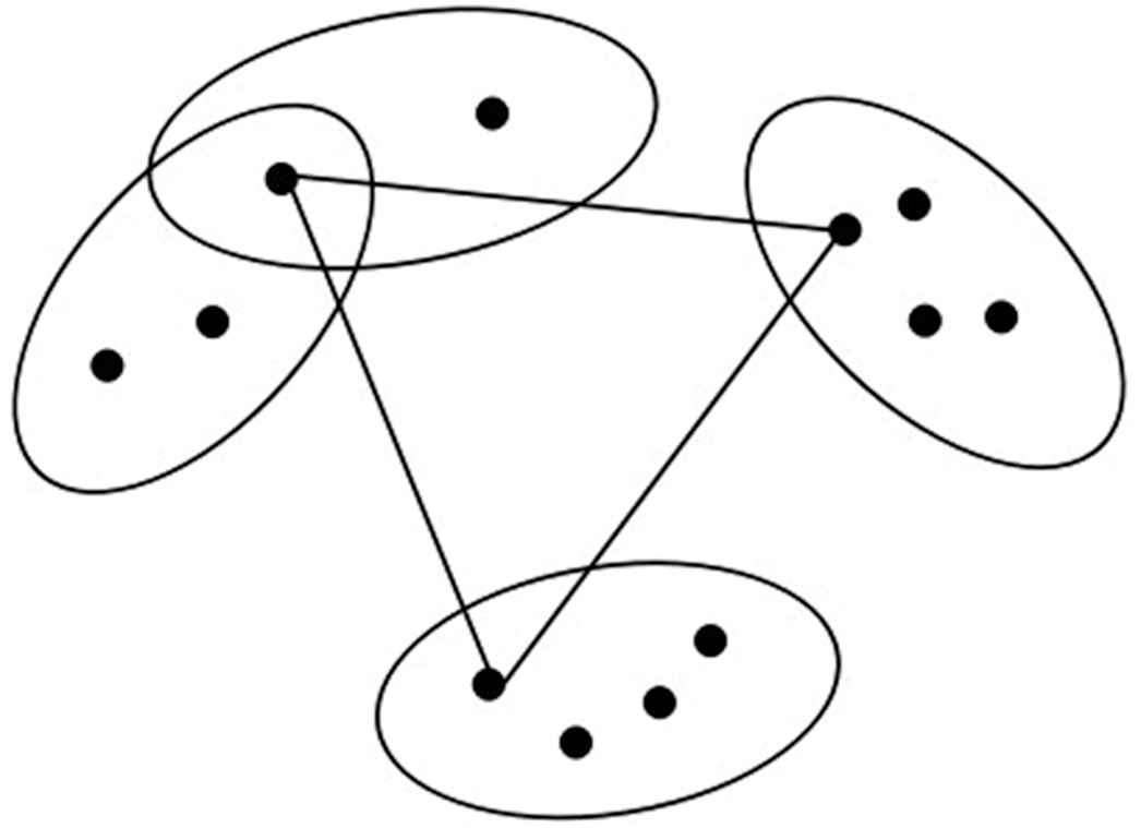
The first kind of generalized traveling salesman problem (GTSP).
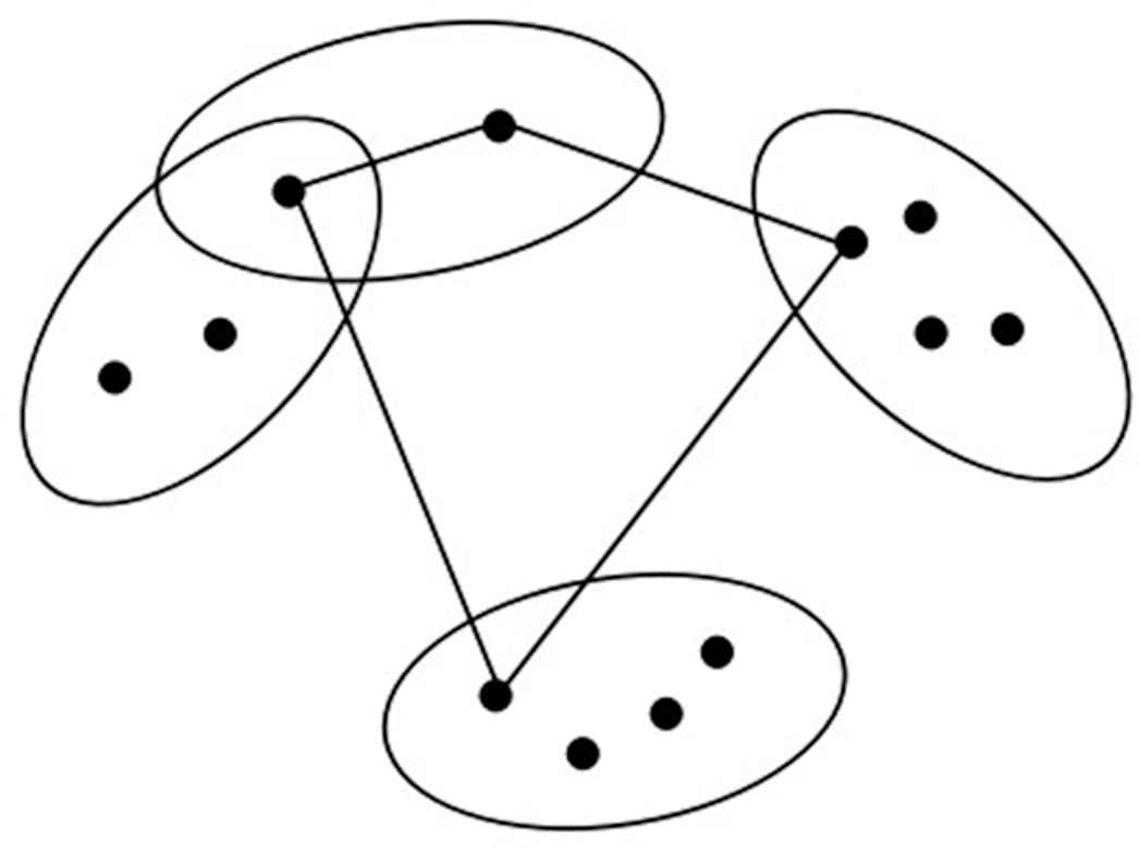
The second kind of generalized traveling salesman problem (GTSP).
The GTSP can be described as follows: let a complete undirected weighted graph
The object function of the GTSP is as follows:
In the 1960s, GTSP was initially proposed by Henry-Labordere [1], Saksena [2], and Srivastava et al. [3] almost simultaneously. So far, there are many practical applications for this problem. Logistics system designs [4], email [5], route planning and naval fleet maritime supply planning [6] are all real-life scenarios of GTSP.
For the first type of GTSP solution, Henry-Labordere, Saksena and Srivastava [1–3] introduced the method of solving GTSP with a simple dynamic programming method. Still, the calculation efficiency of these methods was very low, which can only be used in the case of small problem scale. Then Laporte and Nobert [5] proposed an integer linear programming method with symmetric distance matrix and evaluated the performance of the algorithm using experimental data. This algorithm can solve larger problems than dynamic programming. Laporte et al. [7] discussed the asymmetric GTSP, using relaxation constraints to ensure access to all point groups, and then expanding or modifying the asymmetric TSP by branch and bound algorithm. This improved method increased the problem size to 104 vertices by calculating the results. Fischetti et al. [8] proposed a solution to accurately solve GTSP by using branch and cut, which provides the best solution for an instance of 442 vertices.
Since there are many sophisticated algorithms for TSP solution, some researchers convert GTSP into TSP and then solve it. The current optimization algorithms used to solve TSP problems, such as differential algorithm [9], particle swarm algorithm [10] and ant colony algorithm [11]. Among them, the difference algorithm is more suitable for solving continuous optimization problems and has strong stability. The particle swarm algorithm improves the local search ability of the algorithm when solving TSP, and can better obtain accurate solutions. The ant colony algorithm has also been improved in terms of convergence speed and solution accuracy. Many scholars focus on how to transform GTSP into TSP. For example, Noon and Beat [12] redefined the arc and arc cost of GTSP according to the rules and added a loop within the zero-cost cluster to convert GTSP into an equivalent TSP. Dimitrijevic and Saric [13] proposed to transform the GTSP into an asymmetric TSP with
An effective algorithm will run for a long time as the number of problem nodes or point groups increases. Later, researchers proposed several genetic algorithms (GA) to solve GTSP, and some of them combined local search algorithms with GA to obtain better-operating efficiency. The generalized chromosome genetic algorithm (GCGA) proposed by Wu et al. [15] is by using mixed coding to distinguish the vertices in different groups, and the algorithm generates various feasible solutions through some operations between chromosomes such as crossing and mutation. It then obtains the optimal solution by comparing the loop cost with the function. And in this paper, GCGA is used to solve some examples of processing simple geometric shapes in rectangular plates. In 2006, for the second type of GTSP, Zhao et al. [16] proposed a new GA to add virtual vertices to the generalized chromosome, in which the information of the shortest route between each pair of vertices is reserved in an additional matrix. Wang et al. [17] improved crossover and mutation operators based on the GCGA algorithm and designed a new coding method to obtain a hybrid chromosome genetic algorithm (HCGA). The HCGA uses binary mixed encoding to change the head crossing and increase the possibility of multiple offspring, so the global search effect is better. Snyder and Daskin [18] proposed an effective heuristic algorithm based on the GA. This algorithm improves the solution through random key encoding, and compared with other algorithms improves the quality and running time of the solution in solving the TSP. Ardalan et al. [19] solved the GTSP by making appropriate modifications to the imperialist competition algorithm, using the new coding changes the impact on the cluster and the node selection to produce different results. It has better performance than other algorithms in the benchmark tests of 27 and 40 instances. Kan and Zhang [20] designed an individual mutation method to change the operation of the ant colony optimization algorithm to solve GTSP, and reduced the execution frequency and time complexity of the routing algorithm. Smith and Imeson [21] conducted a research based on adaptive large neighborhood search heuristics. This algorithm has been implemented, and we can find a better solution based on various existing and new problems compared with well-known algorithm tests. Mehdi et al. [22] improved the breakthrough local search (BLS) meta-heuristic and GA to reduce the running time. Experiments show that the improved algorithm can successfully obtain the optimal solution from most research examples.
Up to now, there are many studies on the first kind of GTSP. There are few types of research on the second kind of GTSP. And with the expansion of the scale of the problem, it will become more difficult to solve the problem in polynomial time. On the other hand, DNA computing, as a new intelligent computing algorithm, has two important advantages: huge storage capacity and a large amount of parallelism. A large number of parallel operations can cause chemical reactions of small molecules, and billions of operations can be carried out simultaneously. As a carrier of information, DNA molecules have huge computational storage capacity. Compared with the exponential complexity of other classical algorithms, DNA computing can solve complex optimization problems in polynomial time complexity. Therefore, using DNA computing to solve GSTP will be a meaningful attempt.
We need to obtain an optimal route from the set of all possible routes, and this optimal solution usually has the following restrictions:
All routes are continuous, starting from the specified vertex and ending;
At least one vertex is accessed in each point group, and each vertex is accessed at most once;
The sum of the weights of all routes is the smallest.
Figure 3 shows an example of a graph theory model for a GTSP, in which the eight vertices are divided into three different point groups. In Figure 3, we assume that the travel agent starts from the
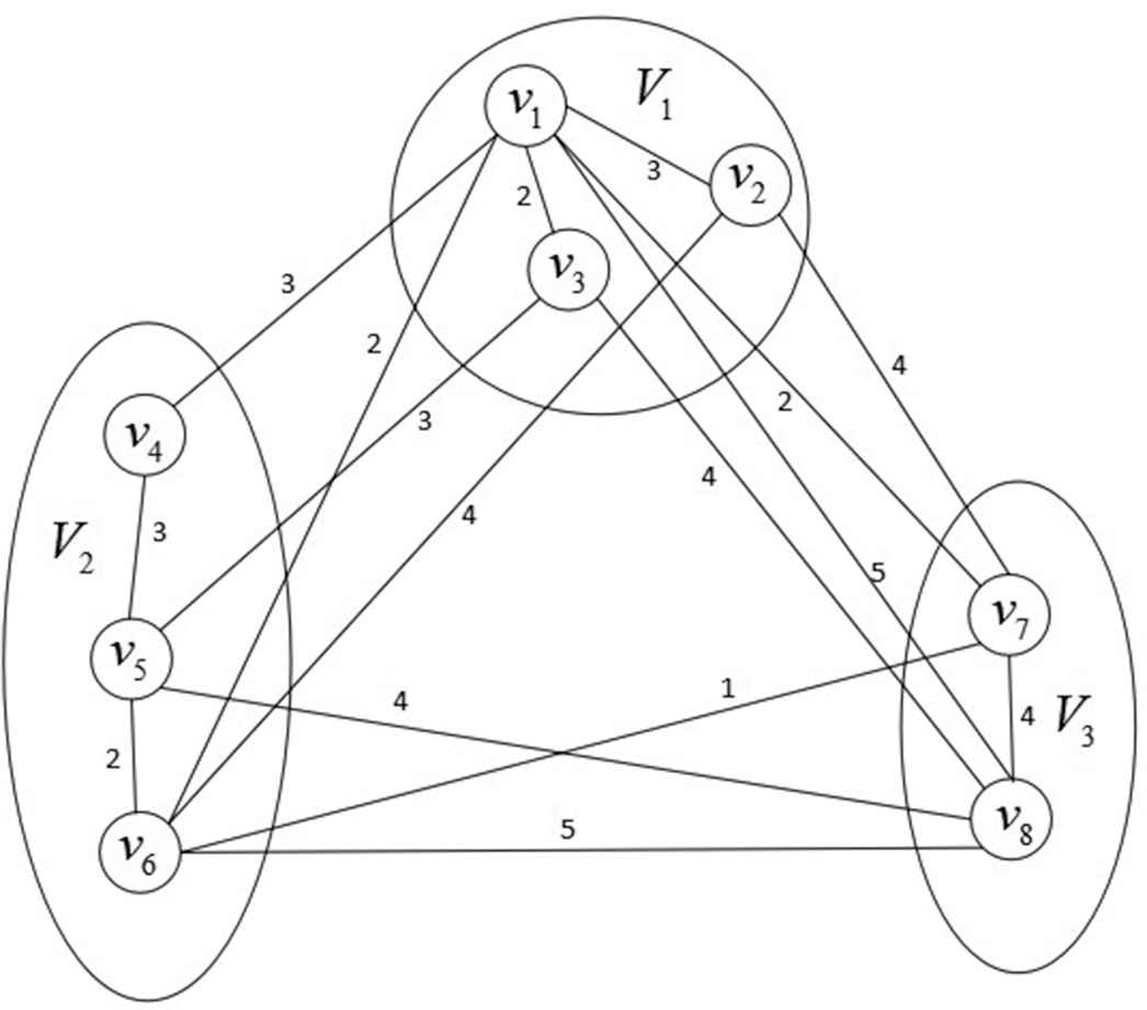
An example of the generalized traveling salesman problem (GTSP) with 8 vertices and 3 groups.
In this paper, for the second kind of GTSP, we propose a DNA algorithm based on the Adleman–Lipton model to solve the GTSP with
The rest of the paper is organized as follows: In Section 2, we review the development of DNA computing and introduce the specific operations of the Adleman–Lipton model. The algorithms and detailed operations of GTSP are presented in Section 3. In Section 4, the feasibility and time complexity of the algorithms are analyzed. Section 5 gives the simulation results of DNA algorithms. The advantages of the DNA algorithm research prospects are considered in Section 6.
2. BACKGROUND KNOWLEDGE
2.1. DNA Computing
DNA molecules in living cells are the leading stores of information. Countless years of biological evolution have improved the molecules and enzymes in the body that can both copy the information in DNA and pass it on to other molecules. DNA is a double-stranded polymer composed of tandem deoxynucleotide chains, where deoxynucleotides are composed of deoxyribose, phosphoric acid and nitrogen-containing bases. The diversity of DNA is due to the random arrangement of base pairs. Different nucleotides base by its definition, respectively for
DNA computing emerged with the rise and development of molecular biology. Biological computing is done by taking advantage of the structure and function of DNA molecules and the parallel operations in their interactions. In the process of continuous development, the advantages of storage capacity and energy consumption gradually emerge. Massive parallelism occurs because molecules interact chemically in tiny volumes and can perform billions of operations simultaneously. Because of the DNA molecule as a carrier of information, calculation of storage capacity is huge. At the same time, the enzymes that perform DNA calculations have been produced over thousands of years of biological evolution and are highly energy efficient. DNA has a broad prospect of resource application. In 1994, Adleman [23] carried out a pioneering work using DNA computing to solve a well-known computational difficulty, namely the directed Hamiltonian cycle problem. As the number of variables increases, the problem becomes more and more difficult. But using DNA computing, the problem can be easy to be solved. The finding proves the feasibility of DNA computing to solve specific problems. Its novelty lies in setting a precedent for applying mathematical problems to calculations at the molecular level, and his pioneering work inspires people. After that, Lipton [24] solved the satisfiability problem based on Adleman's experiment. Qi Ouyang et al. [25] solved the maximum mass problem by using molecular biology techniques. Head et al. [26] solved the problem of maximum independent subset. So far, scientists devoted themselves to the research field of DNA computing and proposed many DNA computing models for NP problems in combinatorial optimization, such as the strand replacement model [27–29], self-assembly model [30,31], tile model [32,33], nanoparticles model [34–36], etc. GA can be used as a tunnel for DNA computing to transform complex optimization problems. Now, with the development of science and technology, GA has been combined with other evolutionary algorithms, such as the gravitational search algorithms (GSAs), particle swarm optimization (PSO) [37,38], etc. These hybrid algorithms have a better hierarchical search function and higher efficiency. At the same time, DNA computing has become the focus of new computing models, which can provide strong technical support for many problems that fail to have effective solutions.
2.2. The Adleman–Lipton Model
Suppose that a series of test tubes contain a limited number of DNA molecules of composed of
Merge
Annealing (T): it can produce all feasible double strands in
Denaturation (T): it can dissociate each double strand in tube
Separation
Discard (T): for a test tube
Copy
Append (T, Z): given a test tube
Selection
Sort
Read (T): given a test tube
Although DNA computing differs from traditional intelligent methods, their computational thinking is the same. Since the above operations can be completed in a limited experimental step, the complexity of each operation can be reasonably set to
3. DNA ALGORITHMS FOR THE GTSP
3.1. Preliminary Ideas
General ideas for conducting experiments using DNA operations are as follows: first, the vertices and point groups corresponding to the GTSP are represented by specific symbols; then, all possible DNA chains of the problem are generated by the biochemical reactions, and feasible chains are selected according to whether different constraints are met; finally, the biological strings corresponding to the optimal solution are obtained by searching and identifying.
It is divided into four steps:
- Step 1:
Construct all possible random routes from the specified fixed node to the end of the same node;
- Step 2:
For all feasible solutions, the route passing through each point group at least once, in turn, is filtered;
- Step 3:
Ensure that each route does not repeat through a node, so that it traverses all point groups once and each vertex at most once;
- Step 4:
By comparing the weights of each route, the optimal result of the GTSP is obtained.
3.2. Notations and Symbols
In this paper, in order to clarify and standardize the expression of our algorithm, it is necessary to define and explain the symbols and notations in the algorithm. Therefore, we use the symbols in Table 1 to illustrate.
| Symbol | Description | Symbol | Description |
|---|---|---|---|
| Vertex set | Edge set | ||
| Weight set | The |
||
| The |
Number of vertices | ||
| Number of point groups | End of DNA strand | ||
| DNA string of the |
point group of the |
||
| DNA string representing weight | DNA string representing point group |
DNA, deoxyribonucleic acid.
Notations and symbols.
3.3. Graph Theory Expression
In the following, we set symbols
3.4. Detailed DNA Algorithms
We will take the GTSP in Figure 3 as an example to introduce the algorithm process in detail.
3.4.1. Generate various possible chains
For a graph with
Algorithm 3.3.1: Generate various routings strands.
- (1-1)
- (1-2)
- (1-3)
- (1-4)
- (1-5)
- (1-6)
- (1-7)
We illustrate the process of the algorithm by taking the GTSP in Figure 3 (starting and ending node is
After the above seven steps, the single chain in tube
3.4.2. Delete routes that do not pass through the point group
There is a limit to the feasible route of GTSP, and at least one vertex in each point group is passed. In other words, if a route does not contain any point group information, then it can't be a viable solution. We remove the unqualified chain by searching the feasible chains.
Algorithm 3.3.2: Select the route passing through each point group at least once.
For
- (2-1)
- (2-2)
- (2-3)
- (2-4)
End for
After this step, we delete the route chains that do not go through all the point groups. We consider in the Figure 3, which the value of
3.4.3. Delete chains that pass through a vertex multiple times
We need to compare the weights of different routes and fill in the vertices in the graph that the route does not pass through. Since we require each vertex to be experienced at most once, we attach chains of information that represent vertices that the route does not pass through. If the length of the chain exceeds a certain length, this means that the corresponding chain represents a route that passes through a vertex multiple times, so the sum of the vertices required for each route should not exceed this limit.
Algorithm 3.3.3: Add vertices information that the route does not pass.
For
- (3-1)
- (3-2)
- (3-3)
End for
- (3-4)
After the above operations, we add the unpassed vertex information to the feasible chain. In Figure 3, we get the number of vertices is eight, and the chain length limit is
3.4.4. Add weight chains for different routes
To select the optimal route, we add the weight chains of corresponding routes to the end of DNA strands. We need to check the weight of the feasible route and then attach the
Algorithm 3.3.4: Add weight chains that the route pass.
For
(4-1)
(4-2-1)
(4-2-2)
(4-2-3)
Else
(4-3)
End for
End for
In Figure 3, after adding the weight chains, the route
Meanwhile, we use two “For” clauses, thus this operation can be finished in
3.4.5. Get the optimal solution chain
The optimal feasible solution chain refers to the minimum sum of edge weights. In the last test tube, we searched for the shortest DNA strands to represent the results of the GTSP. This operation works in O(1) steps.
Algorithm 3.3.5: Search the optimal solutions.
- (5-1)
- (5-2)
We can get the shortest DNA strands for the Figure 3:
So, the shortest route is either
4. CORRECTNESS AND COMPUTING COMPLEXITY OF PROPOSED DNA ALGORITHMS
We demonstrate that the algorithm can obtain the solution of GTSP with
Theorem 1.
The GTSP can be solved by the proposed DNA algorithms.
Proof.
We use different DNA biological chains to represent different vertices, point groups and weights to synthesize complete single strands. By eliminating the unsatisfactory chains in all possible paths, all possible DNA chains are obtained, and then through corresponding DNA operations, the solution to the GTSP is obtained. Specifically, we divided it into five steps: Step 1 generates a set
Theorem 2.
Using DNA molecular algorithms, GTSP can be solved in
Proof.
The complexity of each biological operation is within
Hence, the algorithms solve the GTSP in
5. SIMULATION EXPERIMENT OF DNA ALGORITHMS
In order to prove the feasibility of the algorithm, the simulation experiment is an indispensable part. Our simulation experiments are mainly carried out in three aspects. One is to reasonably design the DNA representation of each element in the problem, which plays a decisive role in the accuracy of the experiment. The second is to reduce the hybridization error rate in the experimental steps to ensure that the corresponding information can be read quickly and accurately. Finally, the process and results of the experiment are presented.
The calculation of DNA depends on the accuracy of the operation of biochemical molecules; otherwise, it will lead to the accumulation and expansion of errors in biochemical reactions. Meanwhile, DNA sequences that may encourage unexpected probe library hybridization should be excluded. Therefore, designing a suitable DNA sequence is a necessary basis for ensuring accuracy with DNA calculations. To achieve these objectives, seven constraints for DNA sequence design were proposed [44]. These limitations include that long homopolymer chains may have unusual secondary structures; if there is no long homopolymer beam, the melting temperature of the probe library mixture will be more uniform; the probe will only bind weakly where it is not intended to bind; and the affinity of the library chain to itself is very low, etc. To this end, we used the sequence design methods in Ref. [44].
In this paper, we use the computational molecular biology tool Biopython as the system development platform, and Braich's program to generate “appropriate DNA sequences” suitable for biological computing algorithm, which can be used to solve the GTSP. Because the original Braich's program did not find the source code of two functions srante48() and drand48(), the standard function srand() was used instead of function srand48() and the source code of function drand48() was added. Our modified program is used to construct a random sequence of 4 bases for each bit of the library, and to check whether the library chain meets the seven constraints of DNA sequence [44]. If the produced DNA sequence does not meet the restrictions, the program will continue to generate another new sequence. When these restrictions can be met, the sequence is accepted for subsequent biochemical reactions. Using this method, we can get the “appropriate DNA sequences” which meets the restriction conditions to improve the accuracy of biochemical reactions [45–48].
Therefore, taking the GTSP (Figure 3) as an example, the program generates random four-base sequences to form
| Bit | Bit | ||
|---|---|---|---|
Sequences chosen to represent
| Bit | Bit | ||
|---|---|---|---|
Sequences chosen to represent the elements
In Table 4, we also calculate the enthalpy, entropy and free energy of the binding of each probe to the corresponding region in the chains. Their average deviation and standard deviation levels are also shown in Table 4. Routes that pass through no more than two vertices of each point group in Figure 3 are shown in Table 5 (due to there are too many possible routes, we only represent some of them). In the simulation experiment, we derive the optimal solution of the GTSP through the composition structure of the last selected DNA sequences in Table 6.
| Vertex | Enthalpy Energy |
Entropy Energy |
Free Energy |
|---|---|---|---|
| 110.5 | 287.7 | 24.6 | |
| 95.1 | 242.9 | 25.1 | |
| 103.3 | 272.1 | 23.6 | |
| 98.4 | 247.3 | 23.3 | |
| 109.6 | 281.1 | 25.9 | |
| 105.2 | 276.2 | 23.1 | |
| 104.5 | 271.9 | 23.2 | |
| 99.7 | 251.3 | 23.1 | |
| Average | 103.288 | 266.313 | 23.989 |
| Standard deviation | 5.356 | 16.791 | 1.075 |
The energies over all probe/library strand interactions.
| Routing | DNA Strands |
|---|---|
Routes that pass through no more than two vertices of each point group in Figure 3.
| Routing | DNA Strands |
|---|---|
DNA sequences chosen to represent the solutions to the generalized traveling salesman problem (GTSP) in Figure 3.
6. CONCLUSIONS
This paper presents DNA biological algorithms for solving GTSP based on the Adleman–Lipton model. In this process, the biological operations are used to produce combined results and to perform screening solutions. Advantages of using DNA algorithms are as follows: first, the algorithms are based on DNA molecules with strong parallel computing power, large storage capacity and low hybridization error rate as we use the specific reasonable coding DNA sequences. Secondly, the proposed algorithms can solve the GTSP at
| Algorithm | Time Complexity |
|---|---|
| DNA algorithm | |
| Garg et al. [50] | |
| Bontoux et al. [51] | |
| Pintea et al. [52] |
Time complexity of different algorithms for generalized traveling salesman problem (GSTP).
In recent years, the research of DNA computing has always been a hot spot. Although there are still some difficulties to be broken through, it is undeniable that DNA has the advantages of storage capability, parallel capability and stability. Further research can consider applying the proposed algorithm to other TSP expansion problems, including mixed Chinese postman problem (MCPP), asymmetric traveling salesman problem (ATSP), generalized covering traveling salesman problem (GCTSP), etc., and trying to establish a unified and standardized model to solve them. We need to explore better ways to combine DNA computing with other computing methods in intelligent systems. We hope that this technological challenge will bring greater progress in science and technology. Moreover, in the development of DNA computing, information recognition, judgment and bio-chain screening can help us to comprehend the origin of computing more deeply, and also promote the process of DNA computing, making it as one of the potential parallel computing methods to solve more complex large data problems.
CONFLICTS OF INTEREST
The authors declare that they have no competing interests.
AUTHORS' CONTRIBUTIONS
All authors contributed to the work. All authors read and approved the manuscript.
ACKNOWLEDGMENTS
It is supported by the Open Research Fund of State Key Laboratory of Simulation and Regulation of Water Cycle in River Basin, China Institute of Water Resources and Hydropower Research (grant No. IWHR-SKL-201905). The project is also funded by research Start-up project of Wenzhou Business School (grant No. RC202002).
REFERENCES
Cite this article
TY  - JOUR
AU  - Xiaomin Ren
AU  - Xiaoming Wang
AU  - Zhaocai Wang
AU  - Tunhua Wu
PY  - 2020
DA  - 2020/12/03
TI  - Parallel DNA Algorithms of Generalized Traveling Salesman Problem-Based Bioinspired Computing Model
JO  - International Journal of Computational Intelligence Systems
SP  - 228
EP  - 237
VL  - 14
IS  - 1
SN  - 1875-6883
UR  - https://doi.org/10.2991/ijcis.d.201127.001
DO  - 10.2991/ijcis.d.201127.001
ID  - Ren2020
ER  -