
A Novel Probability Weighting Function Model with Empirical Studies
- DOI
- 10.2991/ijcis.d.201120.001How to use a DOI?
- Keywords
- Probability weighting function; Decision-making under risk; Lagrange interpolation method; Risk preference; Preference points; Empirical studies
- Abstract
Probability weighting is one of the key components of the modern risky decision-making theories, an effective probability weight function can more accurately describe the decision-makers' subjective response to the event probability. While the probability weighting functions (PWFs) with several different parametric forms and parameter-free elicitation methods have been proposed. This paper first introduces a Lagrange interpolation method (LIM) for building a parameter-free PWF model, then proposes a novel PWF model with the use of the LIM based on Prelec's PWF model. Furthermore, an experiment was designed and carried out. The results not only demonstrate that the novel PWF model could reflect the empirical regularities for maximizing the satisfaction degree of the curve fitting for the preference points obtained from experiment or questionnaire survey and better predict the preferences of decision-makers, but also are found to be consistent with the properties of PWF. This paper makes a significant methodological contribution to developing a numerical method, such as LIM, for constructing the probability weighting model. The finial error analysis suggests that the novel PWF model is a more effective approach.
- Copyright
- © 2021 The Authors. Published by Atlantis Press B.V.
- Open Access
- This is an open access article distributed under the CC BY-NC 4.0 license (http://creativecommons.org/licenses/by-nc/4.0/).
1. INTRODUCTION
Situations that have to make decisions under an uncertain environment are more common than under a deterministic environment. Generally, people have a lot of choices under uncertainty and they may try to understand these choices. Therefore, it is useful to know the decision-maker's underlying preferences. To quantify this choice behaviors process, different theories had been proposed, i.e., an expected utility (EU) theory [1], a subjectively weighted utility (SWU) theory [2], a rank- and sign-dependent utility (RSDU) theory [3], a prospect theory (PT) [4], and a cumulative prospect theory (CPT) [5] have attracted an enormous amount of research attentions in both theories (Refs. [6–9]) and practical applications (Refs. [10–15]).
In a series of decision-making theories under risk and uncertainty, the probability of an event plays a pivotal role in different forms. In the EU theory, the utility of an uncertain prospect is the sum of the utilities of the outcomes, and each weighted by its probability. For example, a prospect
Along with the development of decision-making theory under risk and uncertainty, a large number of scholars began to study the properties and applications of the PWF separately. The properties of PWF were significantly influenced by the source of the event's uncertainty and subjects' risk attitudes. Ref. [18] investigated the relationship between risk attitudes and decision weight. Ref. [19] described the curvature of the PWF, they believed that the PWF permits probabilities to be weighted nonlinearly, and investigated two sources of nonlinearity of decision weights, i.e., sub-additively of probability judgements, and the overweighting of small probabilities and underweighting of medium and large probabilities. At the same time, Refs. [20–22] studied the shape of PWF. Ref. [20] presented a nonparametric estimation procedure for assessing the PWF and value function at the level of the individual subject, and discussed two features of the PWF. Ref. [23] demonstrated that gender differences in risk-taking behavior crucially depend on probabilities. Ref. [24] modeled the effect of people's risk choices by a more curved PWF, research suggests that people are less sensitive to variations in probability in affect-rich compared with affect-poor risky choices. Ref. [25] considered heterogeneity in probability distortion, through experiments, they concluded that 20% of the populations adhere to linear probability weighting, the choice of roughly 80% of the subject exhibit significant deviations from linear probability weighting of varying strength. The proposed PWF model is based on experimental data. Therefore, no matter how many the respondents differ, as long as the preference information is given, the novel PWF model can better reflect and predict respondents' underlying preferences.
Ref. [5] first offered a hypothesis to establish a psychological foundation for the PWF. Based on the weighting function of Ref. [5], Ref. [26] proposed the first axiomatically derived weighting function. Then, Ref. [27] put forward a simpler derivation of Prelec's function. Ref. [28] provided a further simplification derivation of Prelec's PWF. Ref. [29] showed that the Tversky-Kahneman PWF is not increasing for all parameter values and therefore can assign negative decision weighting to some outcomes. Ref. [30] outlined three stylized facts on nonlinear weighting that any alternative theory of risk must address. Ref. [31] utilized psychophysical theory for deriving the Prelec's PWF from psychophysical laws of perceived waiting time in probabilistic choices to study the PWF.
Previous research of PWF could be mainly divided into two parts: parametric PWF and parameter-free elicitation of the PWF. Refs. [5,19,26,32] proposed some descriptive models based on a decision theory, psychology of economic behavior, and experimental data fitting, so these descriptive models are called as parameter PWF models. Furthermore, Ref. [33] provided preference foundations for parametric weighting functions under the RDU. Ref. [34] presented a preference foundation for a two-parameter family of PWF. For the parameter-free elicitation method's research, Ref. [35] devised a simple and direct nonparametric method for measuring the change in relative probability weights resulting from a change in payoff ranks. Ref. [36] provided a parameter-free elicitation of the PWF, used aggregated and individual subject data, and obtained probability weights in a new domain. Ref. [37] proposed an optimally efficient elicitation method which took the inevitable distortion of preferences by random errors into account and minimizes the effect of such errors on the inferred PWFs. Ref. [38] reported the results of an experimental parameter-free elicitation and a decomposition of decision weights under uncertainty. Other studies are focused on making a methodological contribution to experimental development economics (i.e., Refs. [7,39,40]). The focus of this paper is to propose a novel parameter-free PWF model which utilizes a Lagrange interpolation approach and a prelec's PWF to build a parameter-free numerical model. The interpolated preference points are divided into two parts: (a) experimental preference points collected by processing the data of experiment or questionnaire survey and (b) inferred preference points collected by integrating the experimental preference points into the descriptive model (such as prelec's PWF model). The three key steps can be expounded as follows:
The novel PWF model starts with the collection of the experimental preference points. In this process, an experiment or a questionnaire survey is first designed and carried out to obtain several high-quality experimental data, and a group experimental preference points are collected by utilizing certainty equivalent method (it was defined in Definition 2 in Section 2) to deal with the obtained experimental data.
Prelec's PWF model is used to obtain several inferred preference points. In this process, the coefficients of Prelec's PWF model are first determined by curve fitting the experimental preference points. After then, it is easy to use the determined Prelec's PWF model to infer several preference points. Moreover, some mathematical methods are utilized to update these preference points into the inferred preference points.
A Lagrange interpolation approach is introduced to interpolate the experimental preference points and the inferred preference points to build a novel PWF model.
To display the application of the novel PWF model, an empirical study and an error analysis are then carried out in Sections 5 and 6.
The remainder of this paper is organized as follows: Section 2 outlines the preliminaries. Section 3 presents the existing PWF models and analyzes their characteristics. In Section 4, a novel PWF model is proposed to reflect decision-makers' preferences by combining the Lagrange interpolation approach and the existing PWF model. An empirical study is carried out through an experiment survey in Section 5. Section 6 is devoted to analyzing the errors between the proposed model and the existing ones. Finally, Section 7 gives the conclusions and proposes possible extensions.
2. PRELIMINARIES
Being the focus of this paper, the properties of PWF are summarized and redefined as follows:
Definition 1 (Ref. [4]).
PWF
Overweighting for small values of
Underweighting for big values of
Loss aversion. People behave differently on gains and on losses. They are not uniformly risk-averse but distinctively more sensitive to losses than to gains.
A reference point. For different reference points, decision-makers have different subjective responses to the same objective probability
In Definition 1, PWF
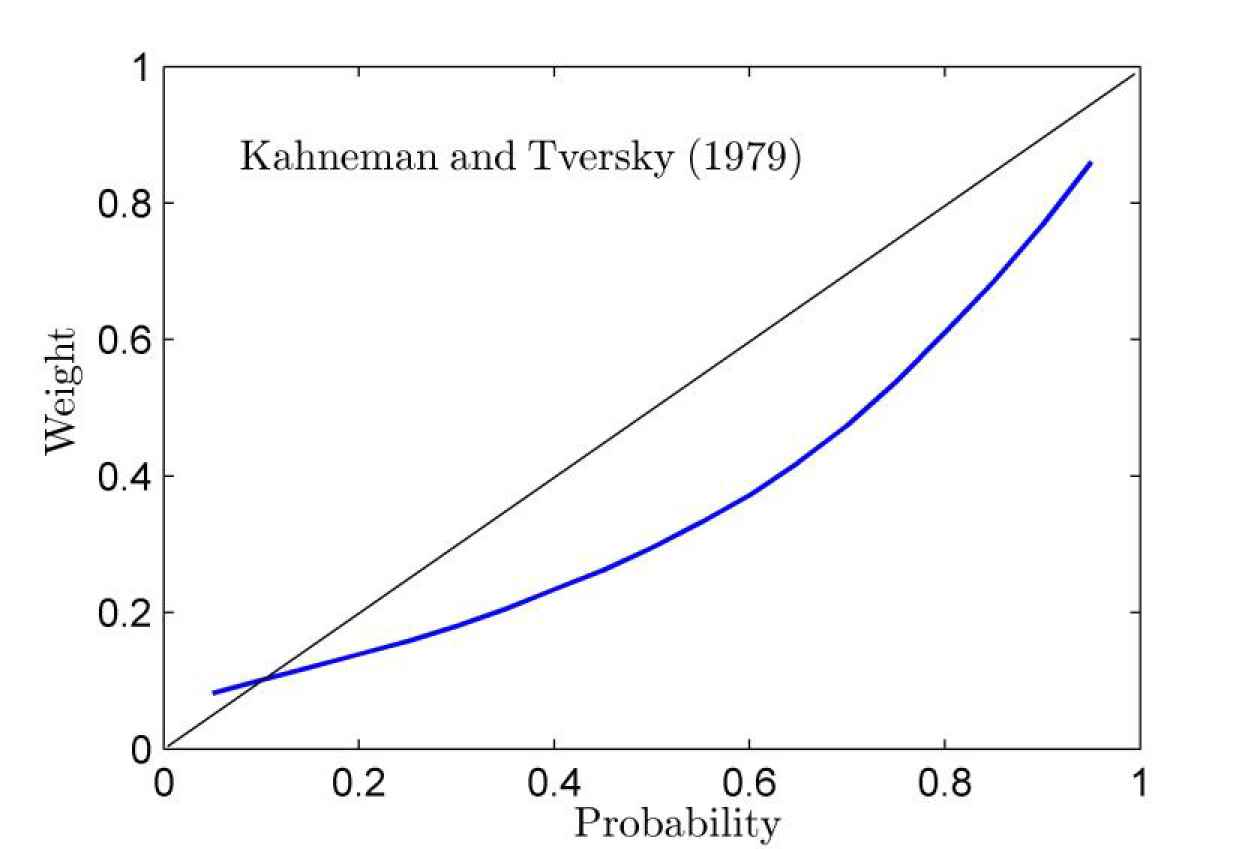
The probability weighting function (PWF) of Ref. [4].
The developments of decision-making theories from the EU to the CPT with gain–loss separability were to accommodate the need of behavioral decision-making. As a result, the value function and PWF are separated. In this process, a value function converts money into value, and a PWF converts a subjective probability into a decision weight. The focus of this paper is on the latter of the two transformations. Through comprehensive reviews of literatures including Refs. [2,19,26,32,34,36,41], it can be found that research of PWF mainly focused on the parametric PWF and the parameter-free elicitation of the PWF. However, the analysis for the two ways both started with obtaining decision weights. To analyze decision weights quantitatively, a certainty equivalent method should be first introduced in order to convert experimental data to decision weights (probability weights).
Definition 2 (Ref. [5]).
For each two-outcome prospect of the form
For convenience, it assumes that
The preference information is denoted as preference points, and the preference points defined as the specific reflection of decision-makers' preferences. In particular, those preference points can be collected by processing experimental data as shown in Section 5.
Definition 3 (Ref. [18]).
The objective probability
The objective probability
The probability weight
The preference points
The preference points are used to reflect the preference of decision-makers, obtain the fitting curve, called preference curve.
The preference points obtained by processing the experimental data are called the experimental preference points such as
The preference points which are obtained by integrating the existing PWF models
Through Definition 3, it can be seen that the preference points are made up of two parts: the experimental preference points and the inferred preference points. The experimental preference points are collected by processing the data of experiment or questionnaire survey as shown in Table 1. The inferred preference points are collected by utilizing the existing PWF models such as those in Table 2 and the experimental preference points to infer.
| Outcomes |
||||||||
|---|---|---|---|---|---|---|---|---|
| Question | Probability | |||||||
| 1.1 | 0.01 | Value | ||||||
| 2 | 4 | 7 | 21 | 46 | 10 | |||
| 1.2 | 0.05 | Value | ||||||
| 0 | 1 | 4 | 5 | 19 | 61 | |||
| 1.3 | 0.10 | Value | ||||||
| 2 | 8 | 3 | 5 | 29 | 43 | |||
| 1.4 | 0.25 | Value | ||||||
| 6 | 3 | 2 | 2 | 38 | 39 | |||
| 1.5 | 0.50 | Value | ||||||
| 7 | 8 | 8 | 35 | 19 | 13 | |||
| 1.6 | 0.75 | Value | ||||||
| 3 | 80 | 4 | 3 | 0 | 0 | |||
| 1.7 | 0.90 | Value | ||||||
| 7 | 11 | 66 | 6 | 0 | 0 | |||
| 1.8 | 0.95 | Value | ||||||
| 10 | 31 | 37 | 8 | 4 | 0 | |||
| 1.9 | 0.99 | Value | ||||||
| 3 | 12 | 62 | 8 | 5 | 0 | |||
Note: The decision data about 90 graduate students are displayed,
Experimental data for prospect
| Model Classifications | Models | Parameters | References |
|---|---|---|---|
| Linear model | Parameter-free | Ref. [1], EU theory | |
| One-parameter model | Ref. [5], PT and CPT | ||
| Ref. [26], PT and CPT | |||
| Two-parameter model | Ref. [43], PT and CPT | ||
| Ref. [26], PT and CPT |
PWF, probability weighting function; EU, expected utility; PT, prospect theory; CPT, cumulative prospect theory.
The existing PWF models.
3. EXISTING PWF MODELS
3.1. Models Review
The development of the PWF can be traced back to the last century (Refs. [4,26,42]). Moreover, with the developments of decision theory, several forms of PWF models, such as a linear model, two one-parameter models and two two-parameter models, have been investigated. These three forms of PWF models recalled in Ref. [8] can be outlined in Table 2.
To analyze the existing PWF models in Table 2, the parameters changes of the PWF models were drawn as shown in Figure 2. By a visual inspection of the shapes of the probability weighting curves, it is not surprising that the PWF curves are both regressive and inverse S-shaped for the value of parameters.
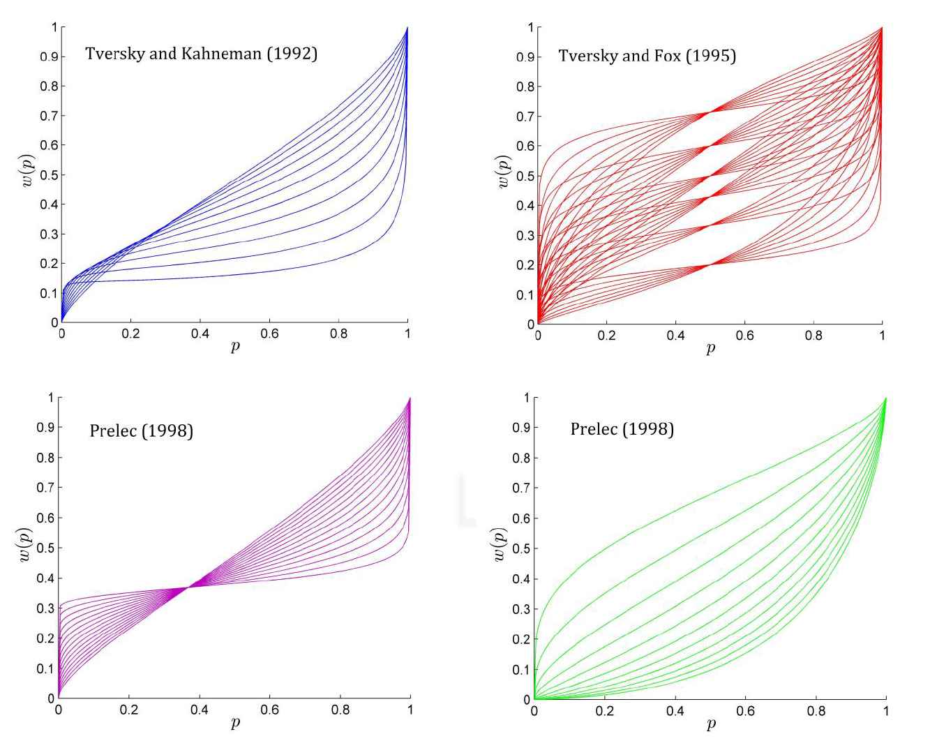
Three families of functions that have been proposed for the probability weighting function (PWF) in prospect theory (PT) and cumulative prospect theory (CPT). Each function is plotted for a range of its parameters: Ref. [5], plotted for different
For these PWF models, the linear model is no parameter, and its curve is a diagonal line; the one-parameter model has a parameter
From Figure 2, it is not difficult to find that how the PWF accommodates three intuitions about the decision impact of small probabilities. Three intuitions are as follows:
It adopts a inverse S-shaped PWF that exhaustively divide the probability interval into a region where the PWF is concave for small probabilities and a region where PWF is convex for moderate and big probabilities.
When the weight of smaller probability tends to 0, the slope tends to infinity at 0, giving a qualitative character to the transition from impossibility to possibility. When the weight of ever bigger probability tends to 1, the slope tends to infinity at 1, giving a qualitative character to the transition from possibility to certainty. The image becomes relatively flatter at smaller probability and bigger probability.
The curvature and elevation of the PWF models are controlled by the models' parameters.
3.2. The Analysis of Advantages and Disadvantages of Existing PWF Models
The analysis in Section 3.1 shows some characteristics such as the inverse S-shaped PWF, the fourfold pattern of risk preferences, and the curvature and elevation of the existing PWF models are controlled by the model's parameters. Generally, more parameters, better to express PWF. However, it is difficult to solve the PWF model when the parameters become more. For this reason, most researchers focused on one-parameter models or two-parameter models. Because the number of the parameters is less, the existing PWF models can be determined using a small amount of experimental data. So it is convenience to obtain a PWF expression under a small amount of preference information about decision-makers. Despite the functional differences between forms of the PWF, they own the same advantage, i.e., using less preference information to obtain a good performance model.
However, the existing PWF models also have some disadvantages. For instance, a parametric estimation makes the models need more assumptions, the assumed functional form has also been determined when a parameter is fixed; if the true functional form is different from the assumed functional form, then it cannot flexibly reflect the preferences of decision-makers. Moreover, the existing PWF models are solved by curve fitting of the experimental preference points, so the solved models can't accurately reflect the choices of the decision-makers. To solve this problem, we first propose the LIM to interpolate the experimental preference points, and then, a novel PWF model is proposed based on the LIM and prelec's PWF model. Therefore, the novel PWF model combines the advantages of prelec's PWF model with the ones of the LIM. Moreover, the novel PWF model can dynamically be response to decision-makers' preferences by adding the preference information into the PWF model once the preference information has been collected.
4. THE PROPOSED NOVEL PWF MODEL
To build a novel PWF model, a group experimental data1 response to the preferences of decision-makers are collected by a relative experiment by conducting the questionnaire survey, and the experimental data are processed to obtain the experimental preference points (the details are presented in Section 5). Here, we present the process of building a novel PWF model, which is derived in two steps. First, the LIM is introduced into interpolating the experimental preference points, and the advantages and disadvantages of this method are discussed in Subsection 4.1. Second, Subsection 4.2 presents a novel PWF model by combining the Lagrange interpolate approach with Prelec's model.
4.1. Lagrange Interpolation Method
A PWF used to reflect and predict decision-makers' underlying preferences is usually built by the curve fitting of preference points. However, the resulting PWF curve does not always go through the preference points, so it can not accurately reflect decision-makers' preferences. The LIM is a numerical method, which has the advantage of constructing a smooth curve which can possibly go through all the interpolation points in a fixed interval using a Lagrange interpolation polynomial [44].
For a certain data points, such as
Lemma 1.
Assume that there are
Then the Lagrange polynomial
It is clear that this polynomial has a degree
Assume that a group experimental preference points
By using the basis function
Note that the numerical model in Equation (11) is a parameter-free model, and it is built by using the LIM to interpolate the experimental preference points that reflect decision-makers' preference. Its advantage is that the functional form can vary according to the information from the experimental preference points. Therefore, the proposed PWF model can dynamically reflect the change of decision-makers' preferences by changing the experimental preference points or its amount. On the basis of the collected experimental preference points
To update the PWF model, the
Based on the basis function
Compared with Equation (11), Equation (14) is changed by adding the
However, the numerical PWF models (11) and (14) also have some disadvantages due to the properties of Lagrange interpolation polynomial. For example, the obtained models would not reflect and predict decision-makers' preferences in an accurate way when the number of interpolation nodes is large or small. On the one hand, the more preference points collected from decision-makers, the more accurate response to preferences of decision-makers. Moreover, the PWF's properties defined in Definition 1 are overweight for small value of
In order to intuitively display the advantages and disadvantages of a numerical PWF model, it is assumed that some experimental preference points such as
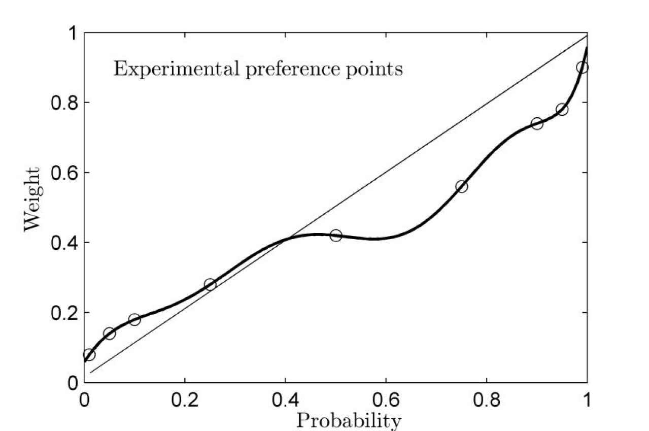
The numerical probability weighting function (PWF) model is built based on experimental preference points.
A good PWF model not only makes accurate response to the experimental preference points possible, but also better predicts the decision-makers' preferences regardless of the amount of experimental data is great or small, as well as satisfying the properties of PWF in Definition 1. To this end, a novel PWF model is proposed to combine the advantages of the prelec's PWF models and the LIM introduced in Section 4.1. Specifically, the novel PWF model is built to utilize the LIM to interpolate the preference points collected by processing the experimental data, and by inferring the preference points from prelec's PWF models.
4.2. A Novel PWF Model
Two cases are considered in the process of building a novel PWF model. At first, it considers the case that the amount of collected experimental data is small. To present the processes of building the novel PWF model, a flow chart is depicted in Figure 4. The two main building blocks of this method are introducing into the prelec's PWF model and updating the preference points. The method begins with conducting experiment or questionnaire survey, ends with obtaining the updated preference points. Then, using the LIM to interpolate the updated preference points, a new PWF model is obtained. For convenience, the novel PWF model is termed as
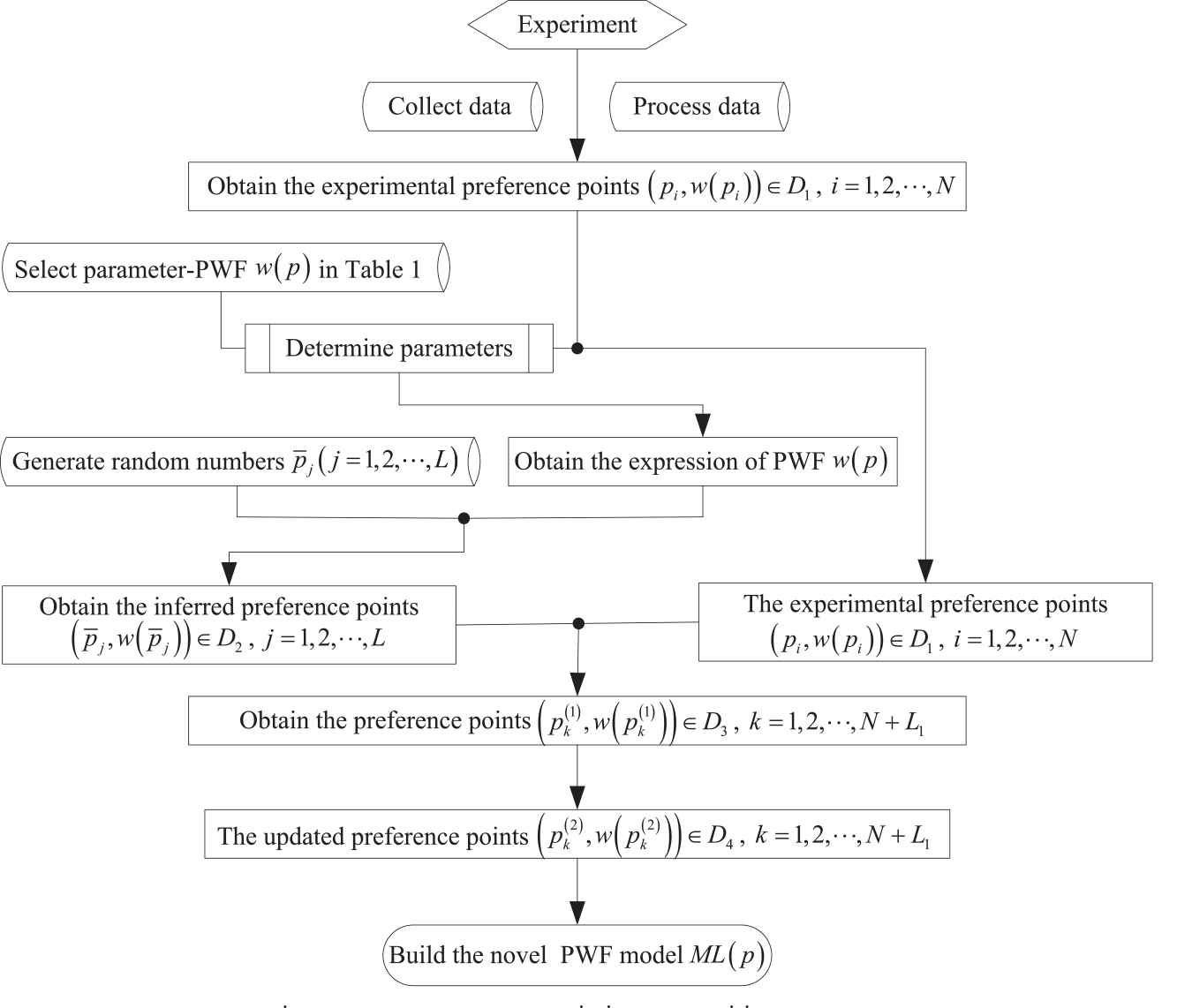
The flow chart of building the modified probability weighting function (PWF) model.
Case 1:
The detailed computation is outlined as follows:
Step 1. Conduct experiments. A set of experimental data is obtained by an experiment or a questionnaire survey (See Section 5.1 for detailed description).
Step 2. Process the experimental data. It first assumes that
Step 3. Select one of the existing PWF models
Step 4. Determine the parameters of the selected PWF model
Step 5. Generate random numbers. To infer the preference information, the random numbers
Step 6. Infer the preference points. Apply the generated random numbers
Step 7. Add the inferred preference points into
If
If we assume that there are
According to the inverse-S property of the PWF [19,20], the function
Step 8. Build the LIM-based model. By using the preference points
Using the interpolation basic functions and the preference points
According to the above 8 steps, the novel PWF model
Case 2:
In this case, a large number of experimental preference points can be collected by using the certainty equivalent approach to process the experimental data. If the proposed approach is utilized to build a PWF model, the built PWF model may be unstable due to the high-order oscillatory of Lagrange interpolation polynomial. To solve this problem, a piecewise Lagrange interpolation approach is proposed. In this process, all steps are same to Steps 1–7 in addition to Step 8 (i.e., a piecewise Lagrange interpolation approach is used in the last step). For instance, it assumes that the updated preference points
The result of dividing the interval into two parts is that the order of the built PWF is reduced by half. If the amount of collected experimental data is large enough, it can also be divided into three parts or more the interval
5. EMPIRICAL STUDIES: APPLICATION OF THE NOVEL PWF MODEL
Several empirical studies have demonstrated the important of PWF and have provided quantitative assessments of its effects (Refs. [5,20]). These studies are consistent with a PWF that satisfies the properties in Definition 1. The aim of the empirical studies in this paper is to examine the proposed novel PWF model's performance. Because of the probability weights are gained by asking a participant for the subjective weight given to a probability (i.e., PWF is the psychological reflects of decision-makers under risk and uncertainty), as they cannot be measured, and must be estimated indirectly through observed choices. Therefore, an empirical study is used to demonstrate the application of the proposed PWF model.
5.1. Experiment Design
An online experiment was designed to collect the preference information of decision-makers under risk and uncertainty. At first, participants were recruited with no special training in decision theory (ss well as the experiments in Ref. [5]). Secondly, the participants were asked to imagine that they were actually faced with the choices described in the questions, and the respondents were asked to indicate the decision they would have made in such a case, separately. For an uncertainty prospect, different decision-makers have different risk preferences, different risk preferences result in different certainty prospects. For this reason, the range of the chosen certainty prospects should be relatively big with a large amount of decision-makers. To solve this problem, the values of certainty prospects is set in a big range3 to induce the respondents to make decision, and the change range of certainty prospects are set according to the properties of PWF in Definition 1. To this end, six options about the certainty prospect's range were given corresponding to an uncertainty prospect in experiment (in generally, the options are three). For convenience, every participant was asked to select one of the six options. The experimental operation interface for the prospect

Example of questionnaire survey for prospect
The experiment consisted of four treatments. Case 1: decision-maker has
5.2. Experiment
The online experiment interviewed 90 graduate students from School of Transportation and Logistics in Southwest Jiaotong University (50 male students and 40 female students). Special efforts were made to obtain the high-quality experimental data by offering a token of appreciation to the respondents for their serious participation in the interview them. The 60-minute online experiment was carried out in a laboratory of the university. Furthermore, the participants were asked to dedicate to the problems of experiment on some computers without communicating with one another.
5.3. Experimental Result
Using statistical software, the distribution histogram of decision-makers' number for the equivalent prospects of prospect
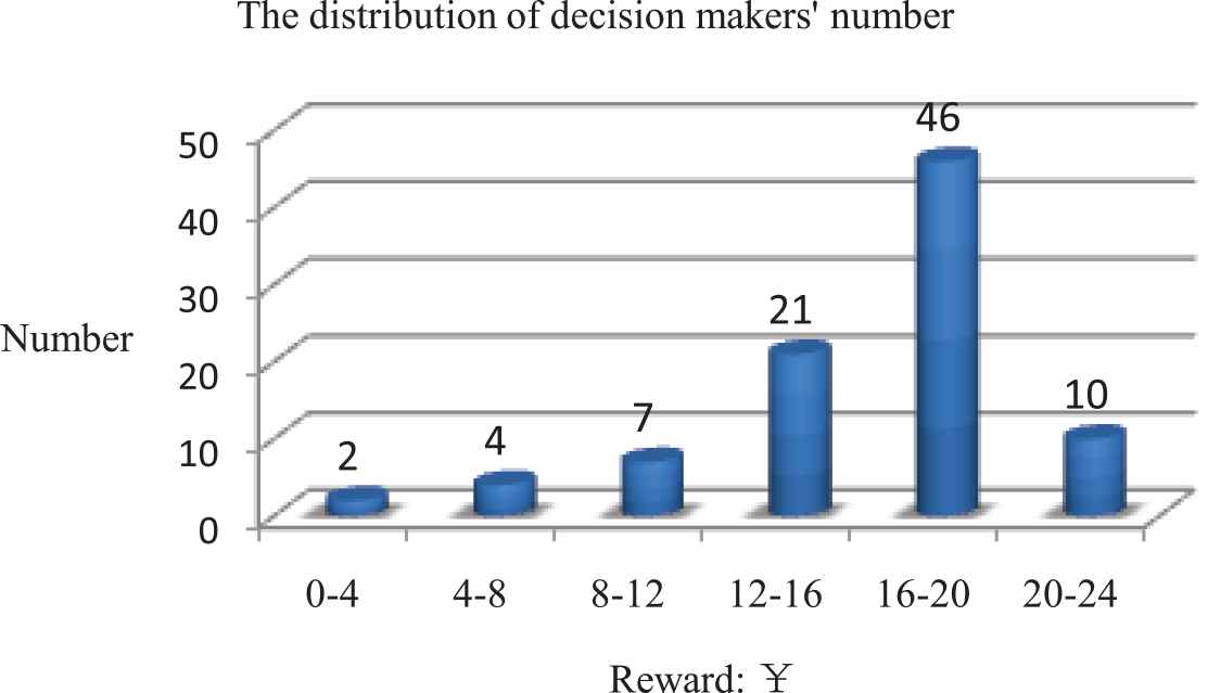
The distribution histogram of decision-makers' number for the equivalent prospects of prospect
Conclusion: 2 respondents chose the option (A) (i.e., the value of
To make experiment more intuitively, it provides a table representation for the case of monetary rewards level in
To obtain the certainty prospects from different probabilities' uncertainty prospects, a transformation was performed to convert a range of certainty prospects to a single certainty prospect using the method described in Equation (25). The computation formula can be given as follows:
| Probability |
|||||||||
|---|---|---|---|---|---|---|---|---|---|
| Outcomes | 0.01 | 0.05 | 0.10 | 0.25 | 0.50 | 0.75 | 0.90 | 0.95 | 0.99 |
| 16 | 28 | 36 | 56 | 84 | 112 | 148 | 156 | 180 | |
| 120 | 240 | 320 | 500 | 760 | 1240 | 1560 | 1640 | 1880 | |
| −6 | −16 | −24 | −48 | −84 | −126 | −160 | −170 | −192 | |
| −100 | −200 | −280 | −420 | −800 | −1240 | −1560 | −1580 | −1900 | |
Note: The two outcomes of each prospect are given in the left-hand side of each row; the corresponding value of median cash equivalents are given in the right columns (i.e., (
Median cash equivalents for all nonmixed prospects.
After experimental data are obtained, Step 1 has been completed, Step 2 then transforms these data into the experimental preference points. Hence, utilizing the certainty equivalent method in Equation (5) to process the experimental data in Table 3, the relationship of objective probability
| Probability |
|||||||||
|---|---|---|---|---|---|---|---|---|---|
| Outcomes | 0.01 | 0.05 | 0.10 | 0.25 | 0.50 | 0.75 | 0.90 | 0.95 | 0.99 |
| 0.08 | 0.14 | 0.18 | 0.28 | 0.42 | 0.56 | 0.74 | 0.78 | 0.90 | |
| 0.06 | 0.12 | 0.16 | 0.25 | 0.38 | 0.62 | 0.78 | 0.82 | 0.94 | |
| 0.03 | 0.08 | 0.12 | 0.24 | 0.42 | 0.63 | 0.80 | 0.85 | 0.96 | |
| 0.05 | 0.10 | 0.14 | 0.21 | 0.40 | 0.62 | 0.79 | 0.83 | 0.95 | |
The relationship of probability
5.4. Empirical Studies
In CPT, the monetary reward
According to Definition 3, the experimental preference points can be collected.
Utilizing the Equation (8), the Lagrange interpolation basis functions
So, the numerical model is built by using the basis function
A modified method is proposed to add the interpolation nodes in Equation (28) so that a novel PWF model can be built by using the updated preference points. To do that, it needs to collect the preference points which are obtained from two parts: one part is from the experimental data processed in Table 4 while the other part is from the inferred preference points. To collect the inferred preference information, Step 3 should be carried out, i.e., a PWF
For the above reason, the two-parameter form analysis model
To generate random number in Step 5, since the number of probability
| Probability and Probability Weight |
|||||||||||
|---|---|---|---|---|---|---|---|---|---|---|---|
| 0.010 | 0.020 | 0.040 | 0.050 | 0.060 | 0.080 | 0.100 | 0.150 | 0.200 | 0.250 | 0.300 | |
| 0.086 | 0.106 | 0.132 | 0.142 | 0.152 | 0.169 | 0.183 | 0.216 | 0.246 | 0.274 | 0.300 | |
| 0.350 | 0.400 | 0.450 | 0.500 | 0.550 | 0.600 | 0.650 | 0.700 | 0.750 | 0.800 | 0.850 | |
| 0.327 | 0.353 | 0.380 | 0.408 | 0.436 | 0.466 | 0.500 | 0.532 | 0.569 | 0.611 | 0.660 | |
| 0.900 | 0.920 | 0.940 | 0.950 | 0.960 | 0.980 | 0.990 | |||||
| 0.718 | 0.747 | 0.779 | 0.798 | 0.819 | 0.871 | 0.909 | |||||
The distribution list of probability
In Step 6, the distribution list of the inferred probabilities
In Step 7, to update the preference points, two small steps are carried out. First, if
| Probability and Probability Weight |
|||||||||||
|---|---|---|---|---|---|---|---|---|---|---|---|
| 0.010 | 0.020 | 0.040 | 0.050 | 0.060 | 0.080 | 0.100 | 0.150 | 0.200 | 0.250 | 0.300 | |
| 0.080 | 0.106 | 0.132 | 0.140 | 0.152 | 0.169 | 0.180 | 0.216 | 0.246 | 0.280 | 0.300 | |
| 0.350 | 0.400 | 0.450 | 0.500 | 0.550 | 0.600 | 0.650 | 0.700 | 0.750 | 0.800 | 0.850 | |
| 0.327 | 0.353 | 0.380 | 0.420 | 0.436 | 0.466 | 0.500 | 0.532 | 0.560 | 0.611 | 0.660 | |
| 0.900 | 0.920 | 0.940 | 0.950 | 0.960 | 0.980 | 0.990 | |||||
| 0.740 | 0.747 | 0.779 | 0.780 | 0.819 | 0.871 | 0.900 | |||||
Note: The bold values represent the unreplaced preference points in Table 5.
The distribution list of probability
Second, the values of the inferred preference points
Then, using the Equation (18), the following values are obtained:
Applying the above method, the part modified preference points are solved as follows:
The total preference points
| Probability and Probability Weight | |||||||||||
|---|---|---|---|---|---|---|---|---|---|---|---|
| 0.010 | 0.020 | 0.040 | 0.050 | 0.060 | 0.080 | 0.100 | 0.15 | 0.20 | 0.250 | 0.30 | |
| 0.080 | 0.101 | 0.129 | 0.140 | 0.149 | 0.165 | 0.180 | 0.217 | 0.249 | 0.280 | 0.308 | |
| 0.350 | 0.400 | 0.450 | 0.500 | 0.550 | 0.600 | 0.650 | 0.700 | 0.750 | 0.800 | 0.850 | |
| 0.336 | 0.363 | 0.391 | 0.420 | 0.445 | 0.471 | 0.498 | 0.528 | 0.560 | 0.611 | 0.669 | |
| 0.900 | 0.920 | 0.940 | 0.950 | 0.960 | 0.980 | 0.990 | |||||
| 0.740 | 0.754 | 0.771 | 0.780 | 0.802 | 0.859 | 0.900 | |||||
Note:The bold values represent the preference points in Table 6 updated using formula (16–20).
The distribution list of probability
Utilizing the 29 preference points in Table 7 to build a novel PWF model, we first solve the Langrage interpolation basis functions
Utilizing Langrage interpolation basis functions
In Equation (36), the PWF model
In order to intuitively display the advantages of the proposed PWF model, the curves of
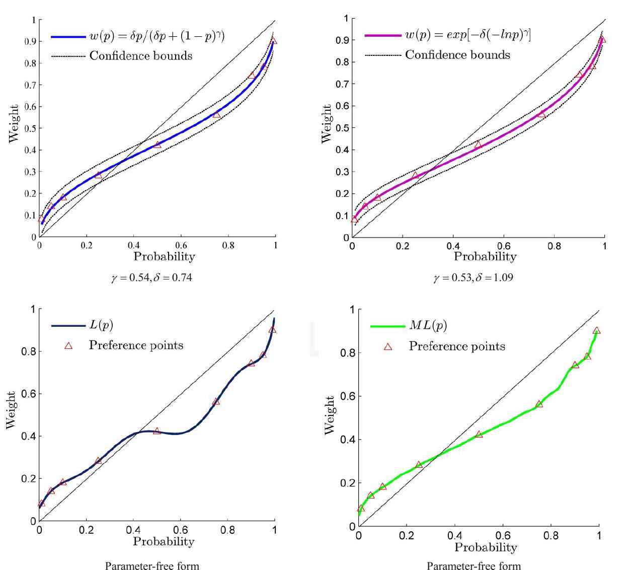
The objective probability
In Definition 1, the properties of PWF are redefined, such as fourfold patterns of risk preferences (properties (2) and (3)), risk-aversion (property (4)), and reference point (property (5)). To explain how the novel PWF model satisfy these properties, the following four cases are compared. Firstly, when the monetary rewards are gains, for small probabilities, decision-makers are more risk-averse at larger levels' monetary rewards (i.e.,
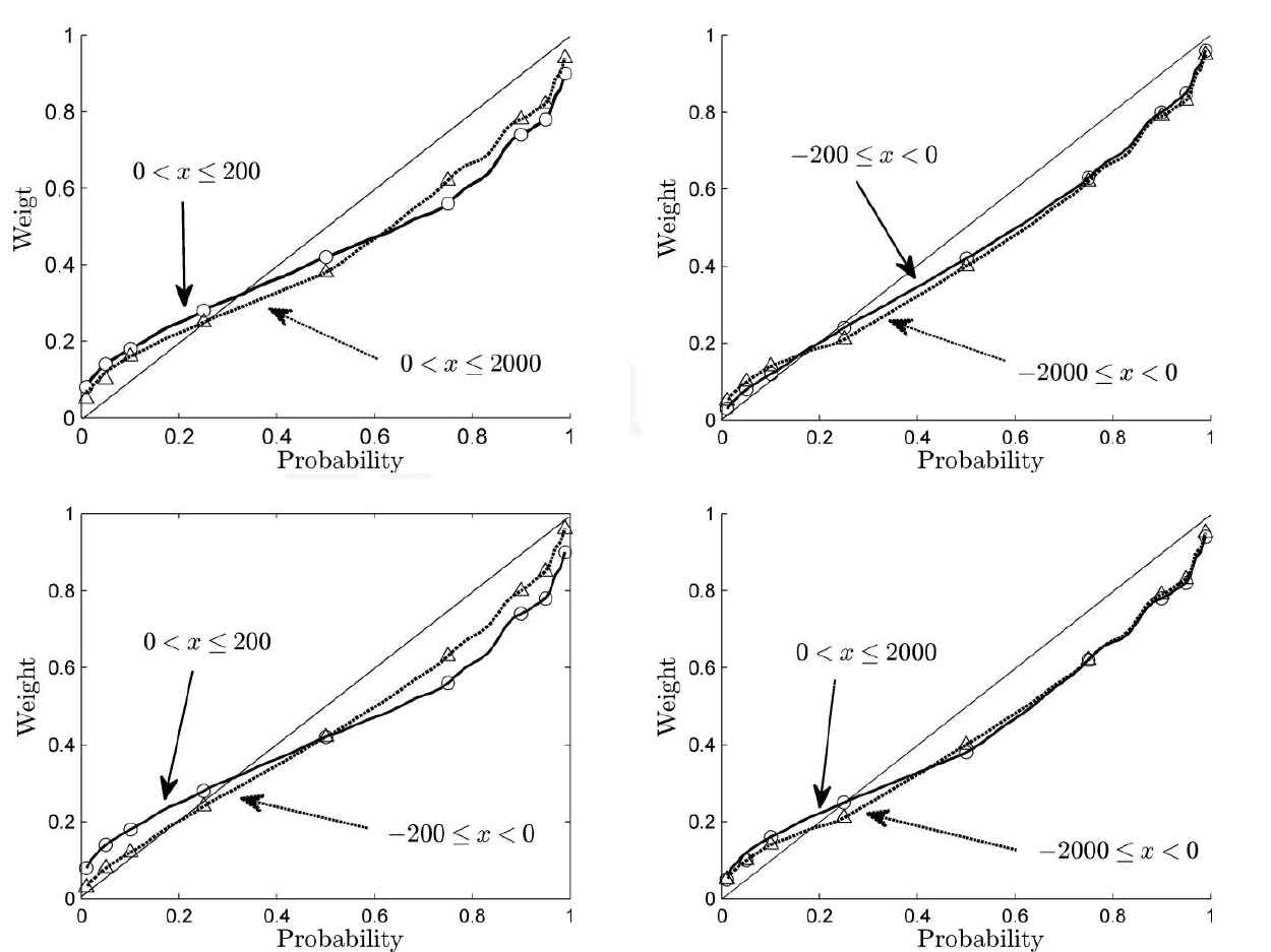
The probability weighting function (PWF) curves with different levels' monetary rewards for gains or losses.
The advantages of the novel PWF model is that its functional form can vary according to information derived from the experimental preference points. To verify this end, we add some new experimental preference points by mean of increasing the number of question subjects, some new experimental data can be obtained and processed. Specifically, the two-outcome prospects with monetary outcomes and numerical probabilities are set in experiment survey. For simplicity, we only consider the cases of monetary rewards
Hence, two new experimental preference points for every level's monetary rewards can be collected respectively. Utilizing the certainty equivalent method to process the above experimental data, the new results can be shown in Table 8 with the thick types representing the new increasing experimental preference information.
| Probability p and Probability Weight w(p) |
|||||||||||
|---|---|---|---|---|---|---|---|---|---|---|---|
| Outcomes | 0.01 | 0.05 | 0.10 | 0.25 | 0.40 | 0.50 | 0.75 | 0.85 | 0.90 | 0.95 | 0.99 |
| 0.08 | 0.14 | 0.18 | 0.28 | 0.33 | 0.42 | 0.56 | 0.70 | 0.74 | 0.78 | 0.90 | |
| 0.03 | 0.08 | 0.12 | 0.24 | 0.35 | 0.42 | 0.63 | 0.72 | 0.80 | 0.85 | 0.96 | |
Note:The bold values represent the preference points added relative to Table 4.
Different levels' monetary rewards corresponding to probability
To build the novel PWF model, the modified method described in Subsection 4.2 is used. Then, in order to express intuitively the advantages, Figure 9 gives the curves of the modified PWF model and the existing PWF model, they are both built by using the new increasing preference points in Table 8. By comparing the modified PWF model
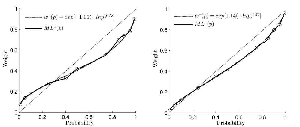
The change curves of the probability weighting function (PWF) by objective probability
6. ERROR ANALYSIS
In existing PWF models, some functions were fitted using the experimental preference points obtained from the experiment or questionnaire survey, their performances are assessed by whether they can provide a reasonably good approximation to both the aggregate and the individual data for probabilities in the range between 0.01 and 0.99 (Ref. [5]). Other functions were proposed by satisfying some axioms and some properties (such as, diagonal concavity, sub-proportionality and compound invariance), their performances were verified by the theoretical analysis (Ref. [26]). In this paper, a novel parameter-free PWF model is built by proposing a numerical approach, and performances analysis is carried out based on errors between the predicted value from the PWF models and the experimental preference points from experiment or questionnaire survey.
Accounting for the effectiveness of the proposed PWF model, some comparisons for the response errors of the existing analysis model [5], the numerical model (such as Equation (21)) and the proposed PWF model (such as Equation (36)) are made. Of course, similar comparisons can be done with some other analysis model (Refs. [5,29,45]), and the results are expected to be the same.
In order to estimate the response errors of different models, the best square estimates are used. The computational formulas are in the context as follows:
In order to present the response error intuitively, the logarithm of the response error
Not surprisingly, the response errors with each model tend to be smaller when the number
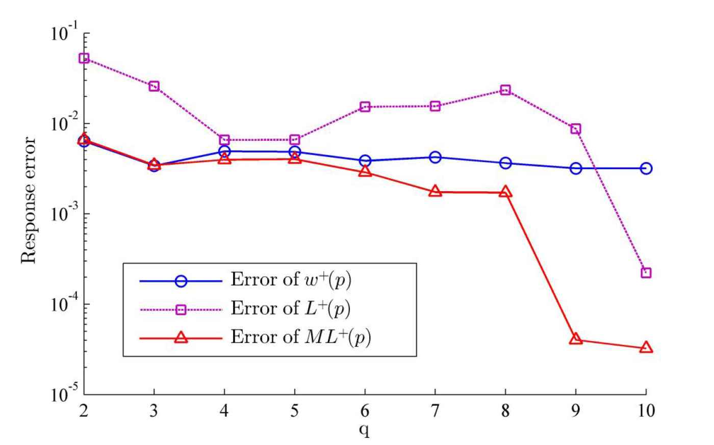
The response errors of the probability weighting function (PWF) for gains in semi-log scale. When increasing the number of the prospect
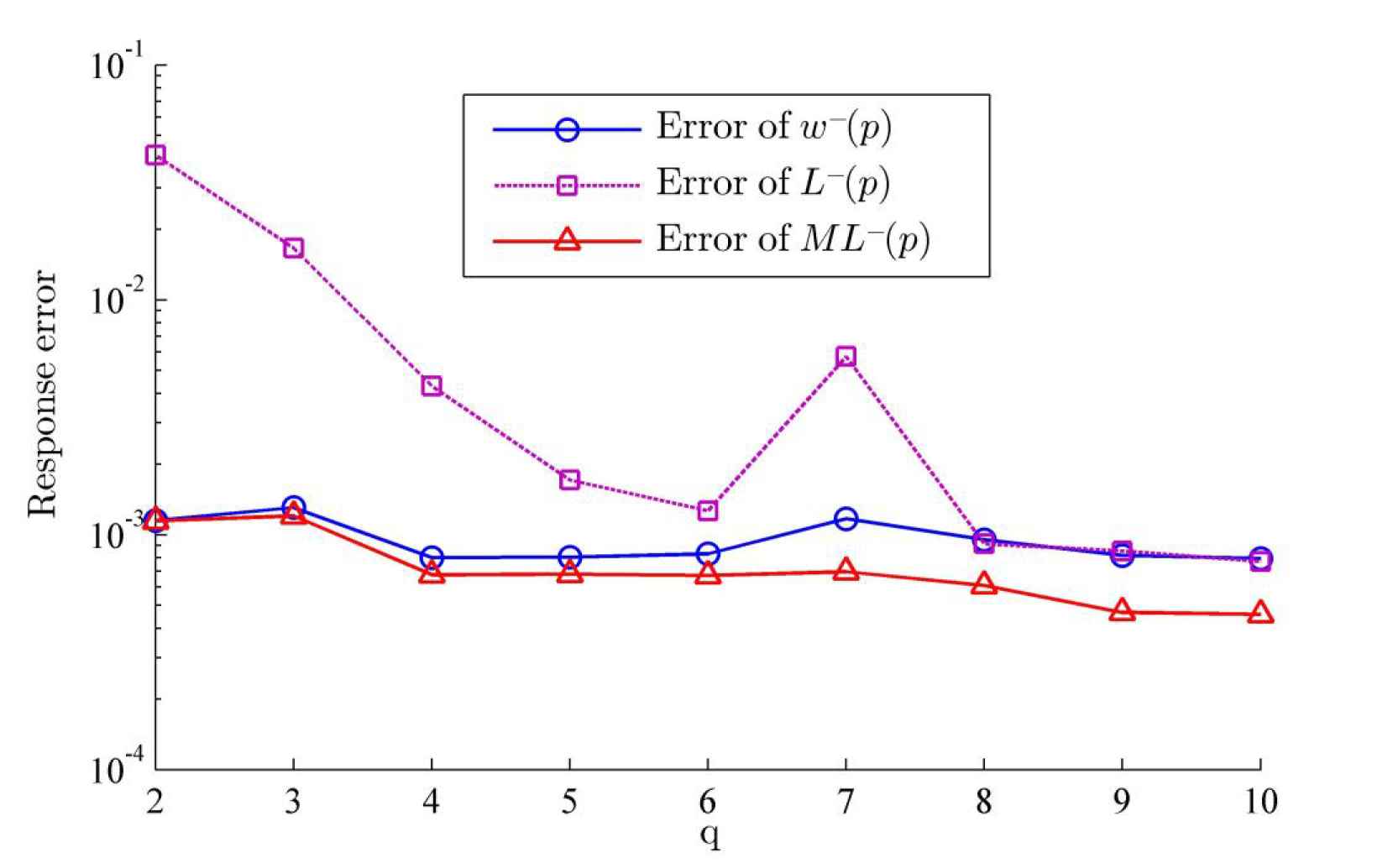
The response errors of the probability weighting function (PWF) for losses in semi-log scale. When increasing the number of the prospect
7. CONCLUSION AND EXTENSIONS
PWFs relate objective probabilities to their psychological weight attached to an outcome, and they play a pivotal role in modeling choices under risk with PT and CPT. In contrast with a parametric form and a parametric-free form of the PWFs, in this paper, we combined the parametric form with parametric-free form by using numerical fitting the experimental preference points and proposed a novel PWF model. The model can not only reflect empirical regularities, but also make the maximum possible satisfaction recent theoretical work. Hence, it can play a very important role in the development of the risky decision-making theory and is better able to reflect a decision's preference for events.
The more preferences information of the decision-makers is collected, and these are high-quality from experiment or questionnaire survey, the more accurate the PWF model is in reflecting and predicting the preferences of decision-makers. Establishing the PWF from a larger population is crucially important yet time-consuming as concluded by Refs. [5,46]. However, improvements in hardware and more efficient programming techniques should be able to solve the above problem. By introducing a numerical method to deal with economy questions, the novel PWF model can be built. At the same time, the error analysis of the novel model has demonstrated that it could not only accurately reflect known preferences of decision-maker, but also better predict unknown preference of decision-makers in a certainty environment (because the preferences of decision-makers are different as the different environment). At last, because of the properties of Lagrange interpolating polynomial (volatility and concussive), some interpolation nodes (i.e., the inferred preference points) are added among the existing interpolation nodes (i.e., the experimental preference points). The modification give rise to more inferred preference points, and help obtain a better performance when the PWF model is built using LIM.
The novel PWF model proposed in this paper is built using LIM when compared to other analysis models shown in Table 2 bring a number of benefits. First, the proposed PWF model can go through the experimental preference points so that it can more accurately reflect the decision-making process. Second, the novel PWF model is flexible as the experimental preference points and their amount change. At last, the proposed PWF model combines prelec's PWF model and numerical model and performs better in predicting the preferences of decision-makers as illustrated in Subsection 5.3.
Detailed explanations have been given on construction and application of the novel PWF model beginning with the collection of experimental preference points, because they are an important component of building PWF model. In other words, if some preference information of decision-makers could not be collected, or the collected preference information are not high quality, the novel PWF model could not be established. However, as long as some preference information of decision-makers is available (even if only a few), the method in Section 4.2 can be applied, and it could build a better performance's PWF model than existing PWF model in Table 2.
This study also suggests several areas for future research. First, as a good performance's PWF model built in PT and CPT is crucially, it would be interesting to apply this novel PWF model in different scenarios, such as option prices (Ref. [47]), lottery decisions (Ref. [10]), inventory problem (Ref. [13]) in risky decision-making. Second, this paper mainly discusses the decision-making in general. More research is required to explore the application of this novel PWF models in the decision-making in individual cases and their applications in weight assignment in the context of multiple criteria decision-making (Refs. [48,49]). Finally, some other numerical methods can be used in researching PWF model.
ACKNOWLEDGMENTS
This paper was partially supported by the progect of Researching on the “Internet plus" WEEE recovery cooperation model and government regulation combination in Henan Province, progect no. 202102310639.
Footnotes
For different reference points, the researchers can obtain different experimental preference points by experiments or questionnaires. Therefore, different numerical PWF model can be built by utilizing Lagrange interpolation approach to interpolate different experimental preference points.
Based on the reasons of psychology, when Giving an uncertainty prospect, participants are difficult to choose an equivalent certainty prospects, but, participants are easy to choose an equivalent certainty prospect in a range. So, we give the certainty prospects' range such as
REFERENCES
Cite this article
TY  - JOUR
AU  - Sheng Wu
AU  - Hong-Wei Huang
AU  - Yan-Lai Li
AU  - Haodong Chen
AU  - Yong Pan
PY  - 2020
DA  - 2020/11/27
TI  - A Novel Probability Weighting Function Model with Empirical Studies
JO  - International Journal of Computational Intelligence Systems
SP  - 208
EP  - 227
VL  - 14
IS  - 1
SN  - 1875-6883
UR  - https://doi.org/10.2991/ijcis.d.201120.001
DO  - 10.2991/ijcis.d.201120.001
ID  - Wu2020
ER  -