
Integrating Grasshopper Optimization Algorithm with Local Search for Solving Data Clustering Problems
 , A. Y. Ayoub2
- DOI
- 10.2991/ijcis.d.210203.008How to use a DOI?
- Keywords
- Data clustering problems; grasshopper optimization algorithm; local search; optimization; swarm intelligence algorithms
- Abstract
This paper proposes a hybrid approach for solving data clustering problems. This hybrid approach used one of the swarm intelligence algorithms (SIAs): grasshopper optimization algorithm (GOA) due to its robustness and effectiveness in solving optimization problems. In addition, a local search (LS) strategy is applied to enhance the solution quality and access to optimal data clustering. The proposed algorithm is divided into two stages, the first of which aims to use GOA to prevent getting trapped in local minima and to find an approximate solution. While the second stage aims by LS to increase LS performance and obtain the best optimal solution. In other words, the proposed algorithm combines the exploitation capability of GOA and the discovery capability of LS, and integrates the merits of both GOA and LS. In addition, 7 well-known datasets that commonly used in several studies are used to validate the proposed technique. The results of the proposed methodology are compared to previous studies; where statistical analysis, for the various algorithms, indicated the superiority of the proposed methodology over other algorithms and its ability to solve this type of problem.
- Copyright
- © 2021 The Authors. Published by Atlantis Press B.V.
- Open Access
- This is an open access article distributed under the CC BY-NC 4.0 license (http://creativecommons.org/licenses/by-nc/4.0/).
1. INTRODUCTION
The classification of similar objects to many clusters (groups) is an idea that has known for a long time. This classification may contain the stars, the elements of chemical, the animals, people, etc. [1]. In the data clustering problem, observations are divided into groups (clusters); where these groups must be homogeneous and the observations in each group are different from the observations in the other groups [2]. Dividing large-size data into similar, homogeneous small clusters helps us to understand and recover them in an easy and efficient way. In addition, these homogeneous clusters give a quick and brief description of the similarities and differences in the original data [3].
The data clustering problem appears in several such fields [4–6]: astronomy, market research, the climate, archeology, bioinformatics and genetics, image analysis, recognition of models (patterns), data compression, retrieval of information, computer graphics, electrical engineering, etc. In addition, it is an important topic for data analysis and exploration.
There are two traditional methods are used for data clustering problems which are namely hierarchical and partitional. These methods have some disadvantages such as (1) empty groups maybe appear in the first step of the solution, (2) sometimes the final division of data is not optimal due to the appearance of extreme points [1–3]. On the other hand, there are many major challenges where many clustering strategies do not work well in data clustering problems due to many factors, such as:
A large number of samples: clustering data problem is NP-hard because if the number of samples to be evaluated is very high, algorithms need to be very sensitive to scaling issues.
High dimensional: If the number of features is very high and exceeds the number of samples, we have to face the curse of dimensional.
Sparsity: Data sparsity greatly impacts calculations of similarity and numerical complexity.
Significant outliers: Finding outliers is highly nontrivial, and removing them is not necessarily desirable.
The swarm intelligence algorithms (SIAs) are usually used for solving this kind of problems (clustering of data), due to the disadvantages of traditional methods. The expression of swarm intelligence (SI) was introduced in 1989 by Gerardo Beni and Jing Wang [7]. SI is an important concept in computer science and artificial intelligence. SI is related to the study of swarms, or colonies of social organisms; where studies of the social behavior in swarms of organisms inspired the design of many efficient optimization techniques. For example, the simulation of bird flocks resulted in the particle swarm optimization (PSO) algorithm [8–11], and the studies the behavior of ants led to the design of the ant colony optimization (ACO) algorithm [12,13].
Since then, many algorithms have been studied that study and simulate swarms such as: artificial bee colony (ABC) [14,15], pigeon-inspired optimization (PIO) [16], monkey algorithm (MA) [17], krill herd algorithm (KHA) [18], bacterial foraging algorithm (BFA) [19], cat swarm optimization (CSO) [20], glowworm swarm optimization (GSO) [21], firefly optimization algorithm (FOA) [22], grasshopper optimization algorithm (GOA) [23], etc.
SIAs and evolutionary algorithms (EAs) are intelligent techniques using as heuristic methods for solving the complex problems that are hard to find its solutions by using normal existing traditional technique [24,25]. They have different structures and worked in different environments. Compared with EAs, the mechanism of sharing information in SIAs is completely different. In EAs, solutions share information with each other which leads to that the whole solutions (population) moves as a one group in the direction of optimal area. But, in SIAs, all solutions converge quickly to the best solution. These algorithms do not always guarantee that they will give the best solution. To improve the ability of these algorithms to solve optimization problems, these algorithms are combined with each other and provide hybrid algorithms [26–28].
There are various SIAs that have been modified to solve data clustering problems. For instance, in El-Tarabily et al. [29] a hybrid algorithm, that combines PSO and subtractive clustering algorithm was proposed to perform rapid classification or clustering for different data sets. In Dai et al. [30], a data combination mechanism was used to improve the ant colony clustering algorithm in terms of computational efficiency and accuracy. Chen et al. [31] proposed a combination between the MA and ABC search operator for clustering analysis; where it was applied to real-life and synthetic datasets. In Abualigah et al. [32], a novel hybrid algorithm between KHA and harmony search (HS) is proposed by Abualigah et al.; where the HS algorithm operator was added to the KHA. Based on CSO, Liu and Shen [33] introduced two clustering approaches (K-harmonic means CSO Clustering and CSO Clustering) to find a suitable classification of data sets. These two methods were presented so that the solution space was explored and exploited and ensures fast access to the optimal distribution of data. Now, it is clear that the clustering of data is an important problem that must be researched and provide a new method with proving its efficiency compared to previous studies.
The GOA is a novel SIAs that is based on the swarming nature of grasshoppers. It mainly depends on the forces of social interaction to find the globally optimum values of the optimization problem. Because of its easy deployment and high accuracy, it is widely used in a variety of industrial scenarios. The main goal of this paper is to introduce a new methodology to solve data clustering problems by using GOA due to its robustness and effectiveness in solving optimization problems. But, GOA has some limitations such as 1) unbalancing between the processes of exploitation and exploration; 2) convergence speed is unstable, and 3) may be fall into the local optimum. So, the local search strategy is applied to enhance the solution quality obtained by GOA and access to optimal clustering for data and overcome the abovementioned limitations.
The main contributions regarding this study are:
A new methodology based on SIA and local search for solving the data clustering problems is presented and evaluated.
A local search strategy to enhance the solution quality and access to optimal clustering of data is applied.
The results of 7 well-known datasets obtained by the proposed methodology are compared with other algorithms.
Stability of the proposed algorithm is verified with the Box chart.
Statistical analysis is used to determine the overall performance of the comparison algorithms.
The remainder of this paper is organized as follows: Section 2: Data clustering problems are illustrated. Section 3: A brief introduction of the GOA is provided. Section 4: The proposed algorithm is described in detail. Section 5: Tests on the proposed algorithm and discussion on results is done. Section 6: a brief conclusion is offered with its future scope.
2. DATA CLUSTERING PROBLEMS
Clustering of data is considered a very important process in many applications as, medical, marketing, business, and social science. Recently, data clustering problems are solved as an optimization problem. So, it is very important to propose a new optimization methodology to solve this problem and introduce a good classification of any data set.
Data clustering problem is the operation of classifying datasets to clusters according to their similarity. In other words, the big data is divided into small clusters so that the elements of each cluster are similar to each other and different from the elements of other clusters. Let us have n points represented by the set
There are many traditional methods of cluster analysis, the most important of which is partitional methods and hierarchical methods. In hierarchical methods, each element is considered a cluster, and then the clusters are combined in a series of successive steps. Hierarchical methods are dividing into [34] divisive clustering and agglomerative clustering. The different methods of hierarchical agglomerative clustering [35] are single linkage, complete linkage, and average linkage. In single linkage, clusters are combined based on the lowest distance between the elements of the two clusters. While, the complete linkage, clusters are combined based on the largest distance between the elements of the two clusters. Finally, clusters are combined based on the average distances between the two elements of the cluster in the average linkage.
On the other hand, the hierarchical methods classify the information into multiple clusters (groups) based on the similarity and characteristics of the data; where the data analysts specify the number of clusters that have to be generated. There are many types of the partitional method, the most famous of which is the k-means algorithm. In the k-means algorithm, the number of clusters is determined and then the centers of the clusters are randomly chosen. The distance between each element and the centers is calculated and based on the lowest distance the element is combined into the cluster. After that, the centers of the clusters are updated based on the average distances between the elements of the cluster and a center. These procedures continue until the number of attempts ends or the cluster centers are not updated.
3. GRASSHOPPER OPTIMIZATION ALGORITHM
GOA is one of the new algorithms for optimization proposed by Mirjalili et al. [23]. GOA is a SIA that simulates the social behavior of grasshoppers in nature to solve optimization problems. The algorithm initially has a population of random (grasshoppers) solutions; where the position of the i-th grasshopper in a d-dimensional space is denoted as
Algorithm 1: The pseudo code of the general GOA.
Randomly initialize positions of all (grasshoppers) solutions.
Set
Do:
Evaluate the objective function value (fitness value).
Determine the best grasshopper (
Update grasshoppers positions according to Equation (1).
Update the decreasing coefficient c according to Equation (2).
While a satisfactory solution has been found.
4. THE PROPOSED ALGORITHM
The proposed algorithm aims to solve the data clustering problems by one of the SIAs: GAO based on local search technique. The proposed algorithm details are described in the following steps:
Step 1: Agents initialization
At generation
Step 2: Distribution of data (points) on clusters
Each point
If there is a solution has empty cluster, it will be regenerated again until no solution that involve empty clusters.
Step 3: Evaluation of agents (centers)
According to the following fitness function (sum of squared error (SSE)), each agent is evaluated:
This function computes the sum of the distances between the points and the center of their cluster.
Step 4: Determine the target center (agent)
The target center (agent) is the agent that give minimum value in the fitness function SSE as:
Step 5: Termination criteria
The algorithm is terminated (go to step 7) either when the maximum number of generation T is achieved or when the N agents of GOA convergences. Convergence occurs when all agents' positions of GOA are identical. In this case, updating the position of each agent will have no further effect.
Step 6: Updating each agent position (clusters centers)
The center of clusters for each agent is updated according to the following equation:
Step 7: Local search
Optimization of the above-formulated fitness function (SSE) using GOA yields an approximated optimal center
Start with an arbitrarily chosen point
Set
Set
Set
The element
If
If
Reduce the step length
whereIf
Establish a pattern direction S as:
and find the new elementwhereIf
If
If
If
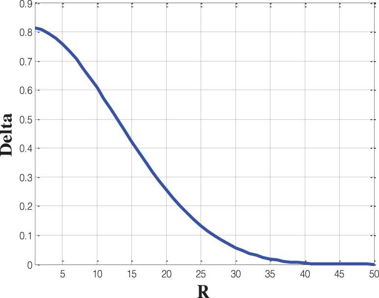
The variation of
Figure 2 shows the flow chart of the proposed algorithm.
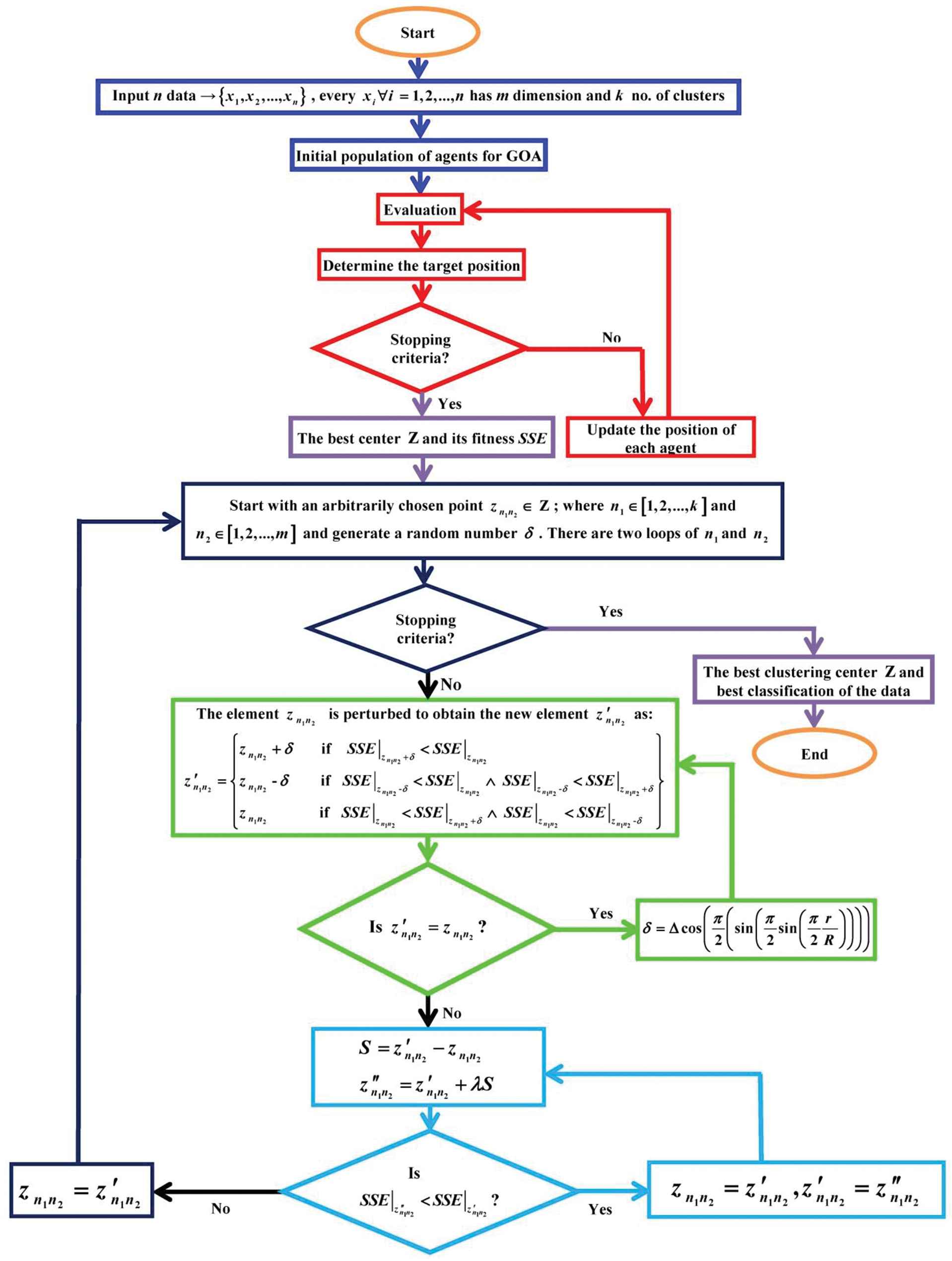
The flow chart of the proposed algorithm.
5. TESTS AND DISCUSSION
In this section, 7 well-known datasets which are commonly used in several studies, are used to test the proposed algorithm and show its power to solve data clustering problems efficiently. These datasets details are shown in Table 1; where their characteristics are provided. All datasets are real-life datasets except Art1 and Art2 are artificial datasets. Classes in the Art1 dataset are distributed according to the following bivariate normal distribution:
| Datasets | Iris | Wine | Art1 | Art2 | Thyroid | cmc | Glass |
|---|---|---|---|---|---|---|---|
| Description | Fisher's iris data | Wine quality data | Artificial data 1 | Artificial data 2 | Thyroid gland data | Contraceptive method choice | Glass identification data |
| Number of clusters | 3 | 3 | 4 | 5 | 3 | 3 | 6 |
| Dimension | 4 | 13 | 2 | 3 | 5 | 9 | 9 |
| Number of data objects | 150 (50, 50, 50) | 178 (59, 71, 48) | 600 (150, 150, 150, 150) | 250 (50, 50, 50, 50, 50) | 215 (150, 35, 30) | 1473 (629, 334, 510) | 214 (70, 76, 17, 13, 9, 29) |
The details of datasets used in experiments.
The proposed algorithm is coded into MATLAB (R2016b) and implemented on a computer with Intel Core i5, 1.80 GHz, and 4 GB RAM. As with any heuristic algorithm, a set of parameters that affect the output of the proposed algorithm is needed. Table 2 displays the parameters managed for the proposed algorithm.
| Number of Agents N | 30–100 |
|---|---|
| Maximum number of iterations T | 10000 |
| l | 1.5 |
| f | 0.5 |
| cmin | 10E-5 |
| cmax | 1 |
| R | 50 |
| Number of runs | 10 |
| Number of clusters | 3–6 |
| Dimension | 2–13 |
| Number of data | 150–1473 |
The parameters of the proposed algorithm.
These datasets are solved by K-NM-PSO [38], ACO [39], ABC [40], PSO [41], enhanced genetic algorithm (EGA) [42], and the proposed algorithm. Our algorithm has been independently run 10 times for each dataset as in other studies [38–42]. The best values, average values and, worst values of the fitness function values (SSE) are recorded after all runs for the six algorithms (see Table 3), which used to evaluate the proposed algorithm stability and accuracy compared to the other algorithms.
| Criteria | Dataset | Iris | Wine | Art1 | Art2 | Thyroid | cmc | Glass |
|---|---|---|---|---|---|---|---|---|
| K-NM-PSO [38] | Average | 97.23 | 16534.52 | 161.08 | 2102.66 | 1986.38 | 5542.05 | 225.95 |
| Best | 97.22 | 16530.54 | 158.51 | 1788.70 | 1966.85 | 5541.64 | 208.95 | |
| Worst | 97.33 | 16550.45 | 184.21 | 2671.54 | 2012.93 | 5544.25 | 250.27 | |
| ACO [39] | Average | 97.34 | 16531.10 | 718.47 | 1940.25 | 1987.19 | 8163.75 | 219.90 |
| Best | 97.22 | 16530.54 | 622.57 | 1836.72 | 1965.81 | 7863.54 | 216.30 | |
| Worst | 97.83 | 16536.19 | 870.18 | 2026.87 | 2008.23 | 8415.07 | 223.12 | |
| ABC [40] | Average | 97.22 | 16530.54 | 158.51 | 1794.86 | 1963.51 | 5542.77 | 214.84 |
| Best | 97.22 | 16530.54 | 158.51 | 1788.70 | 1960.59 | 5541.65 | 208.91 | |
| Worst | 97.22 | 16530.54 | 158.51 | 1850.31 | 1973.04 | 5544.02 | 222.16 | |
| PSO [41] | Average | 97.22 | 16530.54 | 158.51 | 1788.70 | 1960.71 | 5541.64 | 213.41 |
| Best | 97.22 | 16530.54 | 158.51 | 1788.70 | 1960.59 | 5541.64 | 202.92 | |
| Worst | 97.22 | 16530.54 | 158.51 | 1788.70 | 1961.75 | 5541.64 | 226.51 | |
| EGA [42] | Average | 97.11704 | 16527.49959 | 158.148 | 1789.158 | 1950.2411 | 5541.981347 | 213.5787 |
| Best | 97.0395 | 16499.319783 | 157.259 | 1787.623 | 1938.78036 | 5541.36771 | 212.726114 | |
| Worst | 97.3259 | 16555.6794 | 159.568 | 1790.024 | 1978.332887 | 5542.18214 | 216.72251 | |
| Proposed algorithm | Average | 96.6821 | 16483.5207409 | 156.018 | 1735.0988 | 1906.9 | 5534.1290606 | 211.0276 |
| Best | 96.6572 | 16464.6643651 | 155.712 | 1734.5631 | 1895.4 | 5533.1554000 | 210.007073 | |
| Worst | 97.0203 | 16499.3395416 | 157.256 | 1734.5778 | 1938.8 | 5541.3667621 | 212.723411 |
SSE, sum of squared error; ACO, ant colony optimization; ABC, artificial bee colony; PSO, particle swarm optimization; EGA, enhanced genetic algorithm.
SSE values (average, best and worst), for all datasets, that obtained by the different algorithms.
While, Tables 4–10 show the best clustering center obtained by the proposed algorithm during the 10 runs for the datasets: wine, thyroid, iris, cmc, and, glass; where these datasets are real-life datasets. Due to that Art1 and Art2 datasets are randomly generated, the best clustering centers of them are not mentioned. From the tables, we can see that the SSE values obtained by the proposed algorithm, for all datasets, less than those obtained by other algorithms.
| Dataset (iris) | ||||
|---|---|---|---|---|
| Center 1 | 5.937309 | 2.800511247 | 4.419856259 | 1.4199218483 |
| Center 2 | 6.731066 | 3.066509064 | 5.629727780 | 2.1076463368 |
| Center 3 | 5.013232 | 3.404423717 | 1.474707177 | 0.2361141671 |
The best clustering center obtained by the proposed algorithm of the iris dataset.
| Dataset | Center 1 | Center 2 | Center 2 |
|---|---|---|---|
| Wine | 12.89074341415 | 12.53669839860 | 13.659341673748 |
| 2.951722935339 | 2.375857149519 | 1.9568053019164 | |
| 2.382964820629 | 2.329844501169 | 2.4922817456928 | |
| 19.86209932282 | 21.34921254109 | 16.651308927364 | |
| 101.1531859989 | 92.36857306065 | 104.10904591572 | |
| 2.016437539294 | 2.059470449773 | 3.0206994287273 | |
| 1.449738283735 | 1.722567022369 | 3.2150521969562 | |
| 0.394658408539 | 0.441595098429 | 0.3863224228439 | |
| 1.486345632812 | 1.443699035193 | 2.0286503572393 | |
| 5.735783592446 | 4.394498124767 | 5.8283884101347 | |
| 0.910839054293 | 0.936559493928 | 1.0570127951238 | |
| 2.234253759933 | 2.468781689562 | 3.1108583188829 | |
| 721.8570215696 | 464.8171386817 | 1193.1826226275 |
The best clustering center obtained by the proposed algorithm of the wine dataset.
| Dataset (Art1) | ||
|---|---|---|
| Center 1 | −2.9710 | −3.1205 |
| Center 2 | −0.0601 | −0.0232 |
| Center 3 | 2.9896 | 2.9889 |
| Center 4 | 5.9585 | 5.9556 |
The best clustering center obtained by the proposed algorithm of the Art1 dataset.
| Dataset (Art2) | |||
|---|---|---|---|
| Center 1 | 76.6441619814907 | 76.9654703730628 | 77.3768572626618 |
| Center 2 | 48.0164074723632 | 46.6089834004866 | 47.1676176629525 |
| Center 3 | 92.3577280000000 | 92.7229427718792 | 92.5749685959695 |
| Center 4 | 32.7317576855086 | 32.5509020000000 | 32.5327998379686 |
| Center 5 | 62.3938438121938 | 62.8496135066252 | 62.1144830619054 |
The best clustering center obtained by the proposed algorithm of the Art2 dataset.
| Dataset (Thyroid) | |||||
|---|---|---|---|---|---|
| Center 1 | 101.1512 | 9.6290 | 1.9306 | 1.2359 | 1.5369 |
| Center 2 | 114.4504 | 9.5704 | 1.8133 | 1.3506 | 2.3434 |
| Center 3 | 126.9117 | 3.1674 | 0.9267 | 14.5750 | 14.2842 |
The best clustering center obtained by the proposed algorithm of the thyroid dataset.
| Dataset | Center 1 | Center 2 | Center 2 |
|---|---|---|---|
| cmc | 43.717612639902 | 33.4682734976624 | 24.3685883213247 |
| 2.9865987390557 | 3.14880030030017 | 3.00655666885235 | |
| 3.4892950595189 | 3.5647024063982 | 3.5170847091871 | |
| 4.5878463344595 | 3.6286199841112 | 1.7551222933172 | |
| 0.8323635087337 | 0.7888876200036 | 0.9386066588562 | |
| 0.7650568684736 | 0.7083708983022 | 0.7906693108701 | |
| 1.8165191997537 | 2.1013490720444 | 2.3049874066173 | |
| 3.4849637495063 | 3.3059786035364 | 2.9801700728692 | |
| 0.0792896215932 | 0.0688154336252 | 0.0329005419234 |
The best clustering center obtained by the proposed algorithm of the cmc dataset.
| Dataset | Center 1 | Center 2 | Center 3 | Center 4 | Center 5 | Center 6 |
|---|---|---|---|---|---|---|
| Glass | 1.5146 | 1.5173 | 1.5193 | 1.5209 | 1.5299 | 1.5127 |
| 13.006 | 13.314 | 12.842 | 13.102 | 13.809 | 14.637 | |
| 0.0012 | 3.5879 | 3.4595 | 0.2494 | 3.5521 | 0.0649 | |
| 3.0329 | 1.4258 | 1.3069 | 1.4258 | 0.9358 | 2.2096 | |
| 70.619 | 72.671 | 73.015 | 72.682 | 71.854 | 73.269 | |
| 6.2123 | 0.5764 | 0.5885 | 0.3073 | 0.1673 | 0.0468 | |
| 6.9417 | 8.2018 | 8.5687 | 11.989 | 9.5219 | 8.6918 | |
| 0.0013 | 0.0097 | 0.0057 | 0.0509 | 0.0358 | 1.0115 | |
| 0.0015 | 0.0398 | 0.0703 | 0.0566 | 0.0553 | 0.0185 |
The best clustering center obtained by the proposed algorithm of the glass dataset.
On the other hand, due to the SIAs randomness nature, analysis of the Box plot is used to check affirmed of the proposed algorithm stability. Box plot is used to show the difference in the means obtained by the different algorithms used in comparisons. Figure 3 shows the Box plot for all datasets. Figure 3 appears that our algorithm outperformed the other algorithms in terms of stability and optimal of solutions during all runs. This due to that the local search works with GOA to improve the search in the proposed algorithm and achieves a sufficient balancing between exploitative capabilities and explorative tendencies.
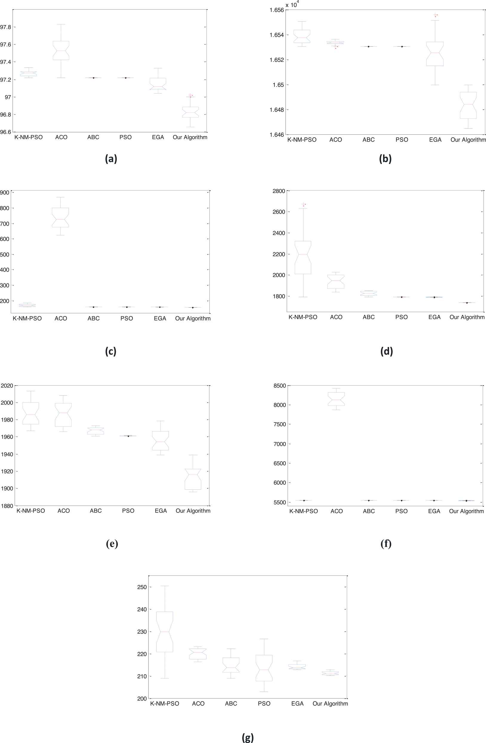
Box plot for all dataset results: (a) iris, (b) wine, (c) Art1, (d) Art2, (e) thyroid, (f) cmc, (g) glass.
5.1. Statistical Analysis
In this subsection, the Friedman statistical test is used to analyze the values of the fitness function (SSE) obtained, for all datasets, using the different algorithms [43]. Also, the Friedman statistical test is performed to show whether the differences in performance between the proposed algorithm and other algorithms used in comparisons are significant or not; where if the Asymp. Sig. (p value) is less than 0.05 which means that there are differences between results obtained by all algorithms. In addition, the Friedman test ranks the algorithms for each dataset separately, and the algorithm that has the best performing obtains rank 1, the second algorithm is in terms of preference obtains rank 2, etc. Then, the Friedman test compares the average rank for the algorithms and determines the Friedman statistics; where the smaller the ranking, the better the performance of the algorithm. Furthermore, pairwise comparisons is performed to illustrate the significant differences between the proposed algorithm and the other algorithms.
Table 11 shows the statistics and mean ranking coefficient of Friedman's test for each clustering algorithm. While Figure 4 shows the mean ranking of the Friedman test on the proposed algorithm and its 5 competitors. From the table, we can see that the p value is 0.000427 (less than 0.05) which means that there are differences between results obtained by all algorithms. In addition, according to the mean rank, the proposed algorithm has a smaller mean rank which means that the proposed algorithm performs better than other algorithms.
| Test Statistics | Method | Mean Rank | |
|---|---|---|---|
| K-NM-PSO [38] | 4.21 | ||
| ACO [39] | 5.43 | ||
| N | 7 | ABC [40] | 3.93 |
| Friedman Chi-squared statistic | 22.465116 | PSO [41] | 3.57 |
| Degrees of freedom df | 5 | EGA [42] | 2.43 |
| Asymp. sig. (P value) | 0.000427 | The proposed algorithm | 1.43 |
ACO, ant colony optimization; ABC, artificial bee colony; PSO, particle swarm optimization; EGA, enhanced genetic algorithm.
Statistics and Mean ranking coefficient of the Friedman's test for each clustering algorithm.
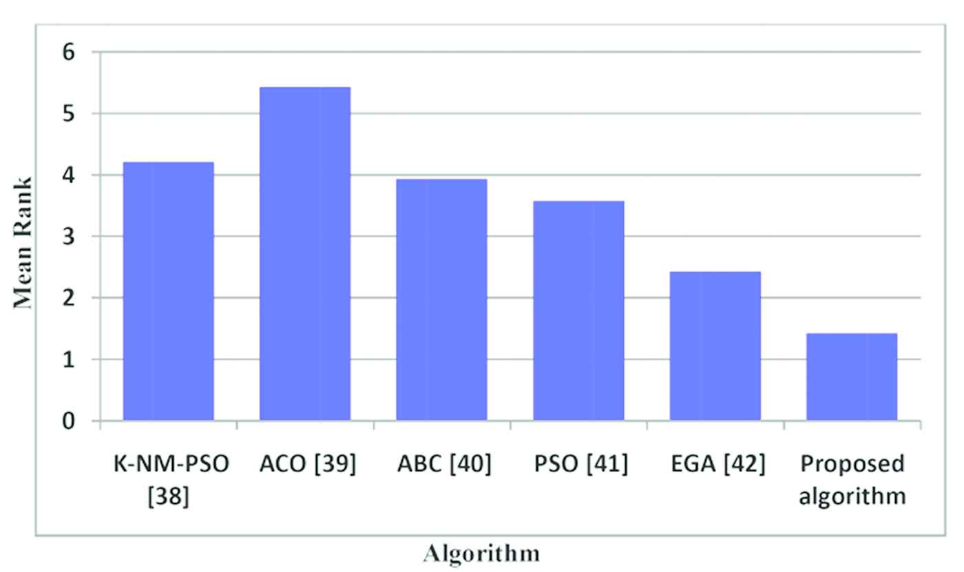
Mean ranking of the Friedman test on the proposed algorithm and its 5 competitors.
Furthermore, pairwise comparisons are performed to illustrate is there a significant difference between the proposed algorithm and the other algorithms or not. Table 12 shows pairwise comparisons between the proposed algorithm and other comparison approaches; where Conover p values, further adjusted by the Holm FWER method, are determined.
| K-NM-PSO [38] | ACO [39] | ABC [40] | PSO [41] | EGA [42] | |
|---|---|---|---|---|---|
| ACO | 0.257617 | ||||
| ABC | 1 | 0.111555 | |||
| PSO | 0.815826 | 0.029725 | 1 | ||
| EGA | 0.036820 | 0.000174 | 0.11156 | 0.27906 | |
| Proposed Algorithm | 0.000463 | 0.000001 | 0.00173 | 0.00876 | 0.367759 |
ACO, ant colony optimization; ABC, artificial bee colony; PSO, particle swarm optimization; EGA, enhanced genetic algorithm.
The proposed algorithm pairwise comparisons (Conover p values, further adjusted by the Holm FWER method).
As shown in Table 12, pairwise comparisons indicate that the proposed algorithm performed statistically significantly better than K-NM-PSO, ACO, ABC and, PSO as the p value is smaller than the level of significance (5%). But there is no statistical significance difference between the proposed algorithm and EGA as the p-value is greater than the level of significance (5%). In terms of pairwise comparisons, it can be inferred that the proposed algorithm is superior to other comparison algorithms for data clustering problems.
6. CONCLUSION
In this paper, a new methodology was proposed to solve the data clustering problems. This methodology used one of the (SIAs: GOA due to its robustness and effectiveness in solving optimization problems. In addition, a local search technique was applied to improve the solution quality and access to the optimal distribution of data. Finally, 7 well-known datasets were used to test the proposed methodology. The proposed algorithm showed several advantages, which we mention as follows:
Using GOA with local search leads to a good balance between global search capability and local search capability to further improve the proposed algorithm performance.
In addition, combined GOA with local search technique accelerates the seeking operation and speeds the convergence to the best distribution of clusters.
Because our procedures are simple, the proposed algorithm can be used to handle large data sets with high dimensions.
The results obtained from our approach have proven to be better than those mentioned in the literature, and it has been proven that they have been successfully applied to solve data clustering problems.
Statistical analysis shows that there are differences between results obtained by all algorithms, the proposed algorithm has the smaller mean rank which means that it performs better than other algorithms and pairwise comparisons indicate that the proposed algorithm performed statistically significantly better than most algorithms that used in comparisons.
In our future works, real applications of data clustering problems should be conducted as machine learning, computer graphics, and image analysis.
CONFLICTS OF INTEREST
The authors declare no conflict of interest.
AUTHORS' CONTRIBUTIONS
All authors are equally contributed in this article.
Funding Statement
This research was supported by the Deanship of Scientific Research at Prince Sattam Bin Abdulaziz University under the research project 2020/01/11812. So, the authors wish to thank Prince Sattam Bin Abdulaziz University, Alkharj 11942, Saudi Arabia, for their support for this research.
ACKNOWLEDGMENTS
The authors would like to thank the referees for valuable remarks and suggestions that helped to increase the clarity of arguments and to improve the structure of the paper.
REFERENCES
Cite this article
TY  - JOUR
AU  - M. A. El-Shorbagy
AU  - A. Y. Ayoub
PY  - 2021
DA  - 2021/02/12
TI  - Integrating Grasshopper Optimization Algorithm with Local Search for Solving Data Clustering Problems
JO  - International Journal of Computational Intelligence Systems
SP  - 783
EP  - 793
VL  - 14
IS  - 1
SN  - 1875-6883
UR  - https://doi.org/10.2991/ijcis.d.210203.008
DO  - 10.2991/ijcis.d.210203.008
ID  - El-Shorbagy2021
ER  -