
Multi-objective Optimization of Freight Route Choices in Multimodal Transportation
- DOI
- 10.2991/ijcis.d.210126.001How to use a DOI?
- Keywords
- Route selection; Multimodal freight transportation system; Risk assessment; Analytic hierarchy process; Multi-objective optimization; Zero-one goal programing
- Abstract
Route selection strategy has become the main aspect in the multimodal transportation system. The transport cost and time as well as the inherent risks must be considered when determining a corrective design plan. The selection of a multimodal transportation network route is a complex multi-objective decision problem. Therefore, considering the impact factors such as the transport cost, time, and comprehensive risk assessment model were further created. This paper develops a decision support model using an analytic hierarchy process (AHP) and zero-one goal programing (ZOGP) to determine an optimal multimodal transportation route. AHP is employed to determine weights of each factor, which rely on expert judgments. The significant weights of criteria obtained from AHP can be integrated in the objective function of ZOGP which is used to generate the optimal route. The empirical case study of coal manufacturing is conducted to demonstrate the proposed model. This methodology can provide a guidance for effectively determining the multimodal transportation routes to improve performance of logistics systems.
- Copyright
- © 2021 The Authors. Published by Atlantis Press B.V.
- Open Access
- This is an open access article distributed under the CC BY-NC 4.0 license (http://creativecommons.org/licenses/by-nc/4.0/).
1. INTRODUCTION
Freight transportation is an important supply chain and logistics aspect. Multimodal transportation has been considered as a major component of modern logistics systems, especially for long-distance transportation and large logistics volumes. Multimodal transportation, as defined by the Multimodal Transport Handbook published by UNCTAD, is the transport of products by several modes of transport from one point or port of origin via one or more interface points to a final point or port where one of the carriers organizes the entire transport. Multimodal transportation is an important development toward making local industry and international trade more efficient and competitive, by its potential to create a smooth flow of goods and better control over the transport chain. Recognizing the benefit of the concept, multimodal transportation has attracted increased attention of late because of ever-increasing road traffic congestion, environmental, and traffic safety concerns. Consequently, many countries have taken initiatives to improve laws and regulations that would create the necessary environment for it to progress. Nowadays, several manufacturers are striving to reduce logistics cost, deliver products on time, minimize freight transportation damage or risks to remain competitive. Therefore, multimodal transportation is currently a key solution of modern transportation systems. Especially, multimodal transportation route selection strategy has become an important component in the logistics of transportation to correctly prioritize multimodal transportation routes.
Solving the freight route choice problem by simultaneously considering the wide range of constraints, including transport logistics cost, transport time, and inherent risk is considered as the most effective approach for generating an optimized freight route choice. In the past, most of the studies on multimodal transportation route selection have emphasized minimizing cost and time only [1–5]. However, there are some studies dealing with minimizing risk[6–9]. Risk is one of the important factors in route selection. It can be associated with accidents, which cause more direct cost, time and reduced quality of logistics systems [9,10]. Additionally, in the case of the transportation and logistics process, the UNCTAD Secretariat stated that risks not only imply a direct cost but also reduce the competitiveness of exports. Therefore, in the decision-making process of transportation route selection, all the three objectives, i.e., cost, time, and risk must be considered in the model.
However, considering all these factors makes route selection a very complex multi-objective decision-making problem. To address this important issue, many scholars have been developing mathematical programing models to optimize route selection to improve the logistics performance. Yang et al. [11]. established a multi-objective optimization model for railway route selection in China. Zhanget al. [12]. proposed a multi-objective optimisation model for route selection of hazardous liquid on the railway network. Although there have been many studies conducted on this issue, but only some studies have addressed optimal route selection for multimodal transportation [9–10]. For example, Meethom and Koohathongsumrit [13] presented an optimization model based on dynamic programing for a container freight transportation.
The aforementioned studies aim was to find the optimal route by considering the various factors in combination with certain optimization algorithms, but as they were based on the established transportation system and also subjectively influenced by field experts when evaluating the importance of weights. Therefore, applying the methods above directly cannot solve the multimodal route selection problem effectively. To mitigate for the shortcoming, it is necessary to utilize a multiple criteria decision-making (MCDM) method including analytic hierarchy process (AHP) to properly weight the coefficients. Kengpol et al. [9]. stated that AHP and an optimization model are a good combination to eliminate the weakness of the transportation problem.
This study developed a multi-objective optimization model, considering transportation cost, time, and risks. It utilized the AHP and zero-one goal programing (ZOGP) to solve the optimal route for the multimodal transportation problem. The practicability of the proposed method is proved by a real case study in Thailand. To validate the model and result, Spearmans rank correlation, and Pearson correlation analysis are carried out on each of the MCDM methods that are studied. Furthermore, sensitivity analysis is also conducted to present the impact on the optimal solution of the proposed AHP-ZOGP model.
The significant contribution of this study can be summarized as follows:
The presented AHP-ZOGP model has competitive performance compared with other techniques for determining multimodal transportation routes. To avoid a large number of pairwise comparisons in AHP method, the proposed model requires the experts to only provide pairwise comparisons on decision criteria. Therefore, the model has no synthesis of pairwise comparison matrices and requires only simple calculation.
The case study is presented along with its contributions to the literature by introducing a holistic list of potential factors affecting the multimodal transportation, including cost, time, freight damaged risk, infrastructure risk, operational risk, security risk, environment risk, law risk, and financial risk. Moreover, the factors in multimodal transportation are identified in two sequential stages using both qualitative and quantitative research approaches. This comprehensive classification not only helps researchers and practitioners identify and classify the potential transportation factors, but also provides a starting point for creating a risk transportation index model applicable to the multimodal transportation process.
This study proposes a route selection framework to reduce bias in risk assessment and to help develop a new decision support system for ranking routes in multimodal transportation. Moreover, the proposed model integrates optimization model minimizing the complexity of cost and time and also uncertainty associated with risk. The study offers useful insights to researchers and practitioners for prioritizing transportation routes as well as optimizing routes under cost, time, and risk decision criteria.
The remainder of this paper is organized as follows: Section 2 presents the literature review. Section 3 explains the methodology and the AHP-ZOGP model is formulated. Section 4 describes the case study and discusses the results. Finally, Section 5 presents the conclusion, limitation, and some efficient directions for future study.
2. LITERATURE REVIEW
Multimodal transportation is a key element within the freight transportation industry [14,15]. It has various definitions; for example, the European Conference of Ministers of Transport in 2001 defined multimodal transportation as the movement of goods in one and the same loading unit or vehicle, which uses successively two or more modes of transport without handling the goods themselves in changing modes. Multimodal transportation is considered as an important development in making local industry and international trade more efficient and competitive. However, the multimodal transport problem has been addressed by many authors [4,5,9,16]. The previous research found that route selection is a fundamental problem of multimodal transportation and logistics management [17,18]. A large number of literature has been published in the area of multimodal route selection. Most of the research studies have focused only on the minimization of cost and time objectives [4,5,16]. However, there appears to be only a few studies dealing with minimizing transportation risk [6–9]. For example, Kengpol et al. [9]. suggested seven key transportation factors; transportation cost, transportation time, freight damage risk, infrastructure and equipment risk, political risk, operational risk, and environment risk.
MCDM methods are approaches to structure information and decision evaluation in formal problems with multiple and conflicting goals [19]. Many authors have applied MCDM methods to solve real-world problems, including the AHP [20] method. AHP is the most popular methodology that has been used in many MCDM problems [21–24]. Because the advantages of AHP are evident. The AHP method transforms a complex multi-criteria problem into a hierarchical structure [24,25] and can be successfully applied to both qualitative data and quantitative data
ZOGP is a technique for MCDM when a decision maker requires to satisfy several goals and to reach the optimal solution [29]. The main advantage of this method is that it has the capacity to handle large-scale problems [28]. Its ability to produce infinite alternatives provides a significant advantage over some methods. However, ZOGP has an inability to weight coefficients. Many applications find its usage necessary in combination with other methods, such as AHP, to properly weight coefficients. This approach allows for proper weighting by eliminating this weakness while still being able to choose from infinite alternatives [28]. Kengpol et al. [9]. combined AHP and ZOGP for a transportation problem. Kim and Emetry [30] and Badri et al. [31]. used ZOGP for a project selection problem.
The previous research studies indicated that the integrated AHP-ZOGP is appropriate and widely used for prioritizing transportation routes. The combined AHP and ZOGP methods can deal with qualitative and quantitative data. Moreover, it is more practical and easier for ranking decisions compared to a large number of alternatives.
Therefore, the proposed integrated AHP-ZOGP model has the following advantages over the methods of absolute priorities [9,10]:
The proposed AHP-ZOGP is more efficient and straightforward than other techniques. The implementation of AHP-ZOGP considers the relative priorities of factor and represents the best alternative. Furthermore, AHP is especially suitable for both qualitative and quantitative modeling. AHP provides a useful mechanism for checking consistency of the evaluation measures and thus reducing bias in decision-making.
This study proposes a methodology that uses a combination of AHP and ZOGP. It is not only to formulate individual models to reach the most suitable output from the viewpoint of each individual expert but also to strike a balance among the possibly different outputs obtained from individual ZOGP model to reach optimal route selection. AHP-ZOGP model have the AHP advantage of generating approximate weights. In addition, ZOGP model are capable of resolving conflict and fulfillment of both tangible and intangible criteria from different experts' view points to achieve the different goals.
The combined AHP-ZOGP model possesses the flexibility of adding new constraints, aspiration levels, improvement objectives or alternative along with resource limitations and modifying them when necessary. However, the integrated AHP-ZOGP model does not have obvious direct disadvantages
The constraints of ZOGP model, such as cost, time and risk limitations, they have only one-to-one relationship between criteria. The aim of these kinds of constraints is not only to take into account the intangible criteria in the model by their quantification using pairwise comparison of AHP, but also to provide a way to measure how well an alternative performs against a criterion. However, ZOGP cannot be used alone because it still requires calculation of the weights of various criteria to use in the objective function of the model. One of the most suitable solutions to this dilemma is to use a combination of AHP and ZOGP in order to obtain a good solution that is close to the ideal one.
3. METHODOLOGY
Appropriate freight multimodal transportation route selection is a strategy to improve the performance of logistics and transportation. To determine the multimodal route selection, we consider the following relevant factors; transportation cost, transportation time, and seven transportation risks. The objective of this research is to formulate a mathematical model that can optimize a multimodal transportation route, which can effectively minimize cost, lead time and transportation risks in a multimodal transportation system. To achieve these approaches, the multi-objective optimisation model can be utilized to obtain an optimal multimodal transportation route. The problem is formulated by using ZOGP. The significant weights obtained from the AHP method are incorporated into the objective function of ZOGP. The significant weights from AHP, parameters and limited data are used to formulate the objective function and constraints. The AHP method and ZOGP are described in the following sub-sections.
3.1. Analytic Hierarchy Process
In the 1970s, Thomas L. Saaty [20] developed the AHP technique, which formulates a decision-making problem into a hierarchy of goal, criteria, sub-criteria, and decision alternatives. AHP has been used in various applications, for examples, road network selection, resource allocation, and evaluation of environmental impacts [32]. In this work, the significant weights of each criterion for each transportation situation are obtained by using the AHP methodology.
In this section, a procedure is proposed to determine the weights of the main criteria, namely transportation cost, time, and the seven transportation risks. We consider the possible coal multimodal routes regarding the main criteria. These criteria, sub-criteria and alternative weights are then calculated. For problem formulation, the following notation is adopted from the general AHP theory. The description of AHP is as follows.
A set of criteria can be assumed as
After the pairwise comparison, a mathematical computation is carried out to establish the relative weights of criteria. The computation includes the calculation of a normalized principle eigenvector from the given matrix
If the rank of matrix
To confirm the certain quality level of a decision, Saaty [20] introduced a consistency index (
Finally, the consistency ratio (
| N | 3 | 4 | 5 | 6 | 7 | 8 | 9 |
|---|---|---|---|---|---|---|---|
| RI(n) | 0.58 | 0.90 | 1.12 | 1.24 | 1.32 | 1.41 | 1.45 |
Random Index (RI) of random matrices [20].
The acceptance limit of
3.2. Zero-One Goal Programing
ZOGP is a well-known modification and extension of linear programming. It became a widely applied technique due to its ability to handle decisions of multiple conflicting goals. However, ZOGP has an inability to weight coefficients. Many applications find its usage necessary in combination with other methods, such as AHP, to properly weight coefficients.
The ZOGP model has been applied very frequently because it is simple to use and understand [33]. This technique is used to minimize the deviation from several objectives because of limited resources. To achieve this, the problem is generally formulated by using the ZOGP model. ZOGP can be used to select the alternatives because of the binary nature of the selection variables and the multiple conflicting criteria involved. In this research, we looked forward to finding the optimal multimodal transportation routes using a multi-objective optimization approach. Owing to the complexity of the transportation data, ZOGP was utilized to solve large-scale problems.
Therefore, ZOGP is now introduced. The purpose of this conceptual model is to avoid the complexity of MCDM problems which includes many decision criteria. This model organizes the decision criteria into clusters with hierarchical structure. The objective function selects the most appropriate alternative from the total deviation of main decision criteria in the highest layer of the model, while the deviation of main decision criteria was computed by constrained functions which are identified deviation between deviation of sub-decision criteria and their maximum deviation.
The proposed route selection model integrates AHP and a multi-objective optimization approach. The significant weights from AHP, parameters, and limited data from previous phases are used to formulate the objective function and constraints. The objective function aims to select the optimal multimodal freight transportation route with the lowest total deviation between route data, minimizing transportation cost, time, and seven important risks. The mathematical formulation of the model is defined in the following equations. The objective function is given in Eq. (5).
The ZOGP methodology can be optimized to obtain a multimodal transportation route. The problem is formulated by using Eqs. (5–18). The significant weights obtained using the AHP method in the previous phase are added into the objective function of ZOGP. The significant weights from AHP, parameters, and limited data from previous phases are used to formulate the objective function and constraints. The definition of multi-objective mathematical optimization model, the indices, parameters, and decision variables are explained below. To clearly present the model formulation, the notation is given as follows:
| Decision Variables | |
| The overachievement deviation of cost | |
| The overachievement deviation of time | |
| The overachievement deviation of freight damaged risk | |
| The overachievement deviation of risk of infrastructure and equipment | |
| The overachievement deviation of operational risk | |
| The overachievement deviation of security risk | |
| The overachievement deviation of environmental risk | |
| The overachievement deviation of law risk | |
| The overachievement deviation of financial risk | |
| The zero-one variables represented the non-selection (zero) or selection (one) of route |
|
| Parameters | |
| The total deviation of objective or main decision criteria for |
|
| The relative weight of cost's objective | |
| The relative weight of time's objective | |
| The relative weight of freight damaged risk's objective | |
| The relative weight of risk of infrastructure and equipment's objective | |
| The relative weight of operational risk's objective | |
| The relative weight of security risk's objective | |
| The relative weight of environmental risk's objective | |
| The relative weight of law risk's objective | |
| The relative weight of financial risk's objective | |
| The coefficient of |
|
| The percentage of transport cost limited by user | |
| The coefficient of |
|
| The percentage of transport time limited by user | |
| The coefficient of |
|
| The percentage of freight damaged risk limited by user | |
| The coefficient of |
|
| The percentage of risk of infra-structure limited by user | |
| The coefficient of |
|
| The percentage of operational risk limited by user | |
| The coefficient of |
|
| The percentage of security risk limited by user | |
| The coefficient of |
|
| The percentage of environmental risk limited by user | |
| The coefficient of |
|
| The percentage of law risk limited by user | |
| The coefficient of |
|
| The percentage of financial risk limited by user | |
The objective functions of ZOGP are combined with the weights from AHP for minimizing the deviation in Eq. (5). The first objective is the transport cost. The second objective is the transport time. The last objectives are the seven multimodal transportation risks. The user could specify the significant weights by using AHP.
The cost constraint in Eq. (6) function represents the deviation between transportation cost and budget. The transport budget should not exceed the user limit. Equation (7) is the time constraint function that is focused on the deviation between transportation time and limited transportation time. Similarly, the transportation time should not be higher than the lead time limited by the user. The constraints for these models are as follows:
Equations (8–14) show the deviation of the seven transportation risks constraint functions that are less than the user limit.
Equations (15–18) create controls to ensure that only one route is optimum for a given situation. If the transportation cost, time, and risks are greater than the user limitations, the route will not be considered.
However, as the data in the objective functions has been recorded in different units, they were converted to percentages (the units for transportation cost, time, and risks are different). The normalization is given by Eqs. (19–23).
4. CASE STUDY AND RESULTS
The multimodal freight transportation system handles a varied range of freight while providing service to a wide range of industries. The major commodity is coal (largely for regional power production), which is one of the world's most important natural resources. It is used in the electricity generating process and other manufacturing industries, such as cement industry, paper industry, and others that require high heat in production. Coal is an unperishable product that is usually transported via waterways, railways, and roads. Therefore, the empirical case study of coal industry is conducted to demonstrate the proposed model. The main objective is to enhance the logistics system's performance by finding the optimal route while minimizing the factors involved.
The research methodology will illustrate the process of data collection and analysis. This study proposed the development of a framework of route selection in multimodal freight transportation, which was then tested on a realistic multimodal transportation problem.
We applied combined methodologies, consisting of AHP and multi-objective optimization. The details of the five-phase framework for route selection in multimodal freight transportation are discussed along with the graphical illustration in Figure 1.
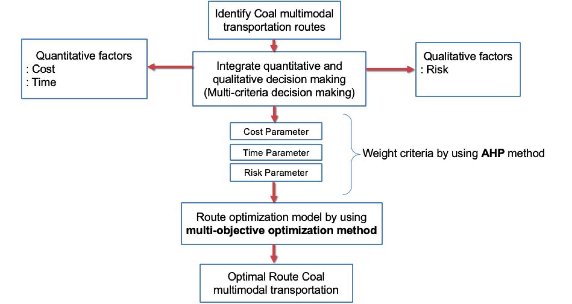
Proposed methodology.
4.1. Scope Definition of Case Study
This section demonstrates the application of the proposal for a conceptual framework for route selection in multimodal transportation with a case study, investigating the domestic freight route in multimodal transportation from Srichang, Chonburi Province in Thailand, to the destination of a cement factory in Saraburi Province, Thailand. These routes are composed of three transport modes, namely, rail, sea, and road.
In this case study, the limitation of capacity is set at 50,000 tons for each possible route. These data can be obtained from interviews and brainstorming of experts and logistics service providers (LSPs). To identify areas of study and appropriate multimodal transportation routes, five experts from three different areas of works associated with multimodal transportation of coal industries were interviewed. From brainstormings and interviews with the experts, eight possible transportation routes were identified (refer to Appendix A). These routes are combinations of several different modes of transport (i.e. rail, sea, and road). In this research, the selection of an optimal multimodal transportation route is based on the multi-criteria that consist of transportation cost, transportation time, and transportation risks.
4.2. Quantitative Data: Transportation Cost and Time
The quantitative data will be represented as the outcomes from certain actions that are measurable in numeric terms. There are two types of quantitative decision criteria in this research, namely, transportation cost and time. The selection of a transport mode or combination of transport modes has a direct impact on transportation cost and time [9].
The transportation cost can be divided into fixed and variable costs. Fixed costs are invariant costs that do not increase or decrease with the size of the transportable product [13]. They are unavoidable transport expenses, including labor cost, depreciation, and insurance cost. Meanwhile, variable costs are avoidable variant costs, such as for trans-shipment, fuel, gate fees and handling charges, and pilotage.
Moreover, the impact of geography mainly involve distance and accessibility. It can be expressed in terms of transportation time. It varies greatly according to the type of transportation mode involved and the efficiency of specific transport routes.
From the possible multimodal transportation routes identified in the previous phase, the selection of transport route has a different impact on transportation cost and time. There are fixed and variable costs associated with multimodal transportation. In this study, transportation cost and time for each possible multimodal transportation route were derived from collecting data through interviewing experts about the actual data. The results are shown in Table 4.
4.3. Qualitative Data: Transportation Risk
This phase is the risk calculation process. Risk analysis is an essential and systematic process to assess the impact, occurrence, and consequences of human activities on systems with hazardous characteristics and constitutes a necessary tool for a safety policy [14]. The first step of risk analysis is risk identification. It is the analysis of the nature of multimodal transportation risk.
This research adopts the non-overlapping risk factors employed by previous research and expert interviews. The risk factors can be assessed in terms of the following criteria:
Freight damage risk. It is identified by using the percentage of damaged goods (value) and loss information. It refers to a situation of a loss of goods or goods damaged during transfer, from transportation, from delivery at a warehouse, or from delivery to a customer [9,10].
Infrastructure and equipment risk. It involves the slope and the width of roads, capacity of roads, trains or ships, risk of shipment in the rainy season, accident rate, and traffic volume. It is the accident rate of each route, quality of road, rail, port, traffic facilities, and equipment material handling in each route [34].
Operational risk. It is defined as a lack of skilled workers, lack of standardization of documents, and interpretation problems with documents or contracts [9,10].
Security risk. The transportation system is a significant consideration in overall transportation planning. Security risk refers to theft from an insider, terrorism, fire, and accidents.
Environment risk. It refers to natural disasters, climate changes, floods, tropical storms, and rainy season carbon released into the air along the multimodal route [34].
Law risk. It means laws, political risk, traffic rules, custom rules, and protesting interference by nearby residents [34].
Financial risk. It refers to financial crisis, fierce competition in the logistics sector, and unattractive markets, for examples, rising cost of fuel, machines and materials, an increase in payrolls, and tax payments in transportation sector in the region and poor financial situation [34].
The second step is risk assessment that is a quantitative risk analysis process. It is used to determine the risk level of an activity by which people, environment, or system might be in hazard. In transportation risk assessment, quantitative risk can be calculated by the probability of accident occurrence multiply with the accident consequence as indicated in Eq. (24) [10,35]:
The potential impact of each risk is indicated on a five-point scale. Tables 2 and 3 present the level of the probability or frequency of accident occurrence (
| Route | Time (Hrs.) | Cost (THB) | Freight Damaged | Infrastructure | Operational | Security | Environmental | Law | Financial |
|---|---|---|---|---|---|---|---|---|---|
| 1 | 73 | 100,501 | 4 | 4 | 4 | 6 | 6 | 2 | 1 |
| 2 | 75 | 109,923 | 4 | 6 | 4 | 4 | 9 | 2 | 1 |
| 3 | 73 | 111,494 | 6 | 6 | 4 | 6 | 9 | 2 | 1 |
| 4 | 75 | 102,070 | 4 | 8 | 12 | 6 | 9 | 9 | 2 |
| 5 | 168 | 94,218 | 4 | 6 | 12 | 6 | 9 | 9 | 2 |
| 6 | 144 | 89,507 | 4 | 6 | 4 | 4 | 6 | 4 | 1 |
| 7 | 99 | 98,929 | 4 | 4 | 4 | 6 | 6 | 4 | 1 |
| 8 | 97 | 95,799 | 6 | 4 | 4 | 4 | 6 | 4 | 1 |
Database of transportation routes.
| Level | The Probability of Accidents Occurrence |
|---|---|
| 1 | No possibility |
| 2 | Small possibility |
| 3 | Moderate |
| 4 | Highly likely |
| 5 | Definitely possible |
Level of the probability of accident occurrence (
| Level | The Consequence of the Accident Impact on LSPs |
|---|---|
| 1 | Not impact at all |
| 2 | Small impact |
| 3 | Moderate impact |
| 4 | Highly likely impact |
| 5 | Definitely impact |
Level of the consequences of the accident (
4.4. Prioritized Criteria by Using AHP Methodology
The AHP method provides a structured framework for setting priorities on each level of the hierarchy using pairwise comparisons that are quantified using 19 scales
Step 1: Construct a complex MCDM problem, which is decomposed into a graphical hierarchy with respect to one or more criteria. The hierarchy is constructed in such a way that the decision goal is at the top level, decision criteria are in the next level and decision alternatives at the bottom. In this study, there are nine criteria in the decision criteria, namely, transportation cost, transportation time, and the seven transportation risks. The AHP Model is as shown in Figure 2.
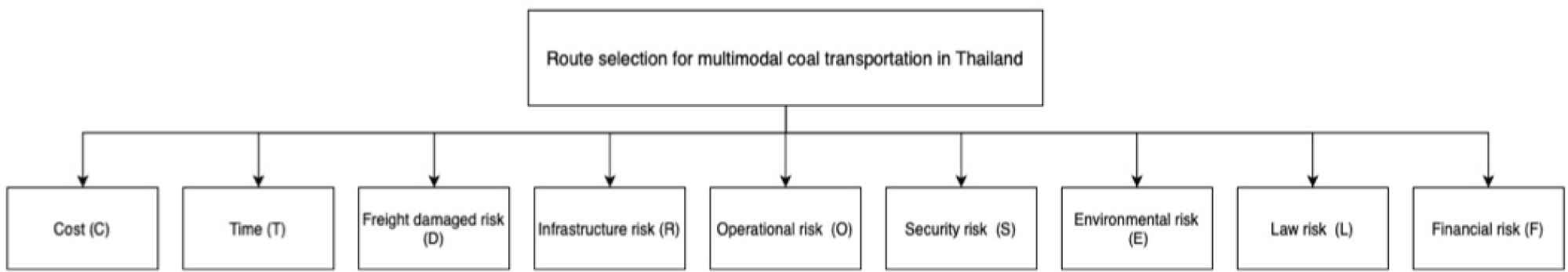
AHP model.
Step 2: Structure the pairwise comparison matrix. Let the pairwise comparison matrix be expressed by the Eqs. (1) and (2). The pairwise comparisons
| Definition | Rating Scale | Reciprocal |
|---|---|---|
| Equally important | 1 | 1 |
| Moderately more important | 3 | 1/3 |
| Strongly more important | 5 | 1/5 |
| Very strongly more important | 7 | 1/7 |
| Extremely more important | 9 | 1/9 |
| Intermediate values | 2, 4, 6, 8 | 1/2, 1/4, 1/6, 1/8 |
The AHP scale suggested by Saaty [20].
Step 3: Calculate the priority weight. The hierarchical priority weight vector is calculated by extracting the eigenvector (
Step 4: Check the consistency. To ensure the consistency of the decision makers preference, the consistency property of the pairwise comparison matrix is applied to check the quality level of a decision. The
The pairwise comparisons between the decision criteria can be conducted by asking the decision maker (DM) or experts which criterion they regard as more important with regards to the decision goal following the score of the AHP scale (Table 5). Suppose a pairwise comparison matrix for the nine assessment criteria provided by the logistics and transportation experts and the answers to these questions form a pairwise comparison matrix which is defined in Figure 3. Through the utilization of Expert Choice software, the resulting relative weight criteria for the transportation cost is 0.260, transportation time is 0.283, freight damage risk is 0.116, infrastructure and equipment risk is 0.069, operational risk is 0.084, security risk is 0.078, environmental risk is 0.041, law risk is 0.046, and financial risk is 0.022. The maximum eigenvalue (

Normalised weight.
4.5. Optimization by Using the ZOGP Methodology
The final phase is to apply the ZOGP methodology to optimize the multimodal transportation routes selection. To achieve this, the problem is generally formulated by using a ZOGP model. ZOGP can be used to select the alternatives because of the binary nature of the selection variables and the multiple conflicting criteria involved. The ZOGP model has been applied very frequently because it is simple to use and understand [33]. The literature as in Kengpolet al. [9]. were specifically chosen for review, as it is a good source of ideas in integrating AHP with ZOGP. The significant weights obtained from the AHP method in the previous stage, associated parameters, and limitations were applied to the objective function of ZOGP [13]. In this case study, the problem is formulated with ILOG CPLEX Optimization. Equations (25–34) can be defined by the deviation variables, decision variables and parameters, respectively (More details in Appendix B). Equations (35–38) ensure that only one route is optimum for each situation. The limitations of each criteria (From experts) are set as constraints that comprise budget not over 110,000 THB, lead time not over 84 hrs, transportation risk score not over 12, and the relative weight criteria from the AHP method as transportation cost at 0.260, transportation time at 0.283, freight damaged risk at 0.116, risk of infrastructure and equipment risk at 0.069, operational risk at 0.084, security risk at 0.078, environment risk at 0.041, law risk at 0.046, and financial risk at 0.022, with
Subject to
In this research, there are nine goals being solved using the ZOGP optimization model. The first goal is that the transportation cost should not exceed the user limit. The second goal is the transportation time not exceeding the time allowed. Finally, the last set of goals are seven multimodal transportation risks that have to be lower than the user's acceptable limits. The deviation variables (
4.6. Comparison with Other MCDM Methods
Comparison of integrated AHP-ZOGP results with other MCDM approaches are conducted to ensure validity and stability of the proposed model and result. The advantage of integrated AHP-ZOGP model is illustrated by its comparison with well-known MCDM approaches. The priority of each factors is determined with those methods to compare with the proposed integrated AHP-ZOGP model. The best-worst method (BWM) [37] and full best-worst method (FUCOM) [38] were employed because the validity of both methods are based on the concept of degree of consistency and pairwise comparison, that are the fundamental of AHP and ZOGP methods.
Each of the selected model was analyzed through the previous discussed models in which BWM-ZOGP and FUCOM-ZOGP model were utilized. For the purpose of validity and stability, the obtained results will present the criteria weight and priority ranking. Table 6 indicates the criteria weight for comparison with other MCDM models–AHP, BWM, and FUCOM–were further employed as input data in the ZOGP model.
| Methods | Transportation Factors |
|||||||||
|---|---|---|---|---|---|---|---|---|---|---|
| C | T | D | R | O | S | E | L | F | ||
| AHP | Weight | 0.260 | 0.283 | 0.116 | 0.069 | 0.084 | 0.078 | 0.041 | 0.046 | 0.022 |
| Rank | 2 | 1 | 3 | 6 | 4 | 5 | 8 | 7 | 9 | |
| BWM | Weight | 0.261 | 0.277 | 0.123 | 0.065 | 0.091 | 0.084 | 0.030 | 0.044 | 0.025 |
| Rank | 2 | 1 | 3 | 6 | 4 | 5 | 8 | 7 | 9 | |
| FUCOM | Weight | 0.255 | 0.290 | 0.133 | 0.065 | 0.091 | 0.077 | 0.032 | 0.045 | 0.012 |
| Rank | 2 | 1 | 3 | 6 | 4 | 5 | 8 | 7 | 9 | |
Alternative criteria weight ranks.
The prioritization discussed previously illustrated that AHP, BWM, and FUCOM models yielded the same weight ranking results in Table 6. However, it can be noticed that these weights are different because of reasons, summarized briefly below:
In the initial stage of determining the weight of AHP, BWM, and FUCOM models, AHP performs
When comparing the pairwise matrix, AHP requires the use of ratio scale, unlike BWM applies integer value. While FUCOM uses any scale (integer or decimal).
The AHP and BWM models rely on mathematical transitivity. However, FUCOM allows satisfying the complete consistency of the model while respecting the conditions of transitivity.
4.7. Result Validation Using Spearman's Rank and Pearson Correlation Coefficient
The correlation analysis is a statistical method used to determine the strength of relationship between two quantitative variables or categorical variables. A high correlation means that two or more variables have a strong relationship with each other whereas a weak correlation means that the variables are hardly related. The values range between −1.0 and 1.0. A correlation of −1.0 indicates a perfect negative correlation, while a correlation of 1.0 indicates a perfect positive correlation. A correlation of 0.0 shows no linear relationship between the movement of the two variables.
Basically, two main types of Spearmans rank correlation coefficient and Pearson correlation coefficient are measured. In this case, Spearman's rank correlation determines the ranked value for each variable, whereas Pearson correlation is used to evaluate the weight score value.
The computation of Spearman's rank correlation and Pearson correlation are based on the following definitions [39]:
Spearmans rank correlation coefficient:
wherePearson correlation coefficient:
Correlation
The results from Spearmans rank correlation coefficient and Pearson correlation coefficient analysis, shown in Figure 4, confirm the validity of the proposed AHP method. The AHP is most highly correlated with the weight ranking whereas the BWM method is least correlated with the weight ranking. Therefore, AHP method make evident that the ranking of criteria weight remain steady and produces the best overall results.

Correlation between the results of the criteria weight and ranking.
4.8. Sensitivity Analysis
Sensitivity analysis, also known as simulation analysis or the what-if analysis, determines the robustness of a model's outcome. It studies the effect of independent parameters on dependent parameters. The independent variables are varied over a range, and its effect on the outcome is observed. Sensitivity analysis discusses the impact of changing in the parameters of an ZOGP optimization model. Sensitivity analysis increases the confidence in the proposed AHP-ZOGP model, by providing an understanding of how model respond to change in the inputs. The sensitivity analysis is carried out by changing the cost, time, and freight damaged risk by +/-5 to 20 %. In this analysis, these factors are selected due to highest weight respect to other factors.
From the results as shown in Tables 7–10, the sensitivity analysis indicated that the output of AHP-ZOGP model does not change much, it is said to be insensitive or robust although the factors are decreased and increased by +/−20 %. On the other hand, the results from BWM and FUCOM indicate that the output varies noticeably when changing the input variables from minimum to maximum over a range, then the output is said to be sensitive.
| Factors | Methods | Cases | Results |
|---|---|---|---|
| Cost | AHP-ZOGP | Decreased by 5% | Route 1 |
| AHP-ZOGP | Increased by 5% | Route 1 | |
| BWM-ZOGP | Decreased by 5% | Route 2 | |
| BWM-ZOGP | Increased by 5% | Route 2 | |
| FUCOM-ZOGP | Decreased by 5% | Route 1 | |
| FUCOM-ZOGP | Increased by 5% | Route 1 | |
| Time | AHP-ZOGP | Decreased by 5% | Route 1 |
| AHP-ZOGP | Increased by 5% | Route 1 | |
| BWM-ZOGP | Decreased by 5% | Route 1 | |
| BWM-ZOGP | Increased by 5% | Route 1 | |
| FUCOM-ZOGP | Decreased by 5% | Route 1 | |
| FUCOM-ZOGP | Increased by 5% | Route 1 | |
| Freight damaged risk | AHP-ZOGP | Decreased by 5% | Route 1 |
| AHP-ZOGP | Increased by 5% | Route 1 | |
| BWM-ZOGP | Decreased by 5% | Route 1 | |
| BWM-ZOGP | Increased by 5% | Route 1 | |
| FUCOM-ZOGP | Decreased by 5% | Route 1 | |
| FUCOM-ZOGP | Increased by 5% | Route 1 |
+/− 5 % sensitivity analysis result.
| Factors | Methods | Cases | Results |
|---|---|---|---|
| Cost | AHP-ZOGP | Decreased by 10% | Route 1 |
| AHP-ZOGP | Increased by 10% | Route 1 | |
| BWM-ZOGP | Decreased by 10% | Route 2 | |
| BWM-ZOGP | Increased by 10% | Route 3 | |
| FUCOM-ZOGP | Decreased by 10% | Route 4 | |
| FUCOM-ZOGP | Increased by 10% | Route 2 | |
| Time | AHP-ZOGP | Decreased by 10% | Route 1 |
| AHP-ZOGP | Increased by 10% | Route 1 | |
| BWM-ZOGP | Decreased by 10% | Route 3 | |
| BWM-ZOGP | Increased by 10% | Route 2 | |
| FUCOM-ZOGP | Decreased by 10% | Route 1 | |
| FUCOM-ZOGP | Increased by 10% | Route 1 | |
| Freight damaged risk | AHP-ZOGP | Decreased by 10% | Route 1 |
| AHP-ZOGP | Increased by 10% | Route 1 | |
| BWM-ZOGP | Decreased by 10% | Route 2 | |
| BWM-ZOGP | Increased by 10% | Route 3 | |
| FUCOM-ZOGP | Decreased by 10% | Route 3 | |
| FUCOM-ZOGP | Increased by 10% | Route 3 |
+/− 10 % sensitivity analysis result.
| Factors | Methods | Cases | Results |
|---|---|---|---|
| Cost | AHP-ZOGP | Decreased by 15% | Route 1 |
| AHP-ZOGP | Increased by 15% | Route 1 | |
| BWM-ZOGP | Decreased by 15% | Route 4 | |
| BWM-ZOGP | Increased by 15% | Route 4 | |
| FUCOM-ZOGP | Decreased by 15% | Route 3 | |
| FUCOM-ZOGP | Increased by 15% | Route 2 | |
| Time | AHP-ZOGP | Decreased by 15% | Route 1 |
| AHP-ZOGP | Increased by 15% | Route 1 | |
| BWM-ZOGP | Decreased by 15% | Route 6 | |
| BWM-ZOGP | Increased by 15% | Route 5 | |
| FUCOM-ZOGP | Decreased by 15% | Route 2 | |
| FUCOM-ZOGP | Increased by 15% | Route 2 | |
| Freight damaged risk | AHP-ZOGP | Decreased by 15% | Route 1 |
| AHP-ZOGP | Increased by 15% | Route 1 | |
| BWM-ZOGP | Decreased by 15% | Route 4 | |
| BWM-ZOGP | Increased by 15% | Route 3 | |
| FUCOM-ZOGP | Decreased by 15% | Route 6 | |
| FUCOM-ZOGP | Increased by 15% | Route 6 |
+/− 15 % sensitivity analysis result.
| Factors | Methods | Cases | Results |
|---|---|---|---|
| Cost | AHP-ZOGP | Decreased by 20% | Route 1 |
| AHP-ZOGP | Increased by 20% | Route 2 | |
| BWM-ZOGP | Decreased by 20% | Route 3 | |
| BWM-ZOGP | Increased by 20% | Route 3 | |
| FUCOM-ZOGP | Decreased by 20% | Route 4 | |
| FUCOM-ZOGP | Increased by 20% | Route 2 | |
| Time | AHP-ZOGP | Decreased by 20% | Route 1 |
| AHP-ZOGP | Increased by 20% | Route 2 | |
| BWM-ZOGP | Decreased by 20% | Route 4 | |
| BWM-ZOGP | Increased by 20% | Route 5 | |
| FUCOM-ZOGP | Decreased by 20% | Route 5 | |
| FUCOM-ZOGP | Increased by 20% | Route 5 | |
| Freight damaged risk | AHP-ZOGP | Decreased by 20% | Route 1 |
| AHP-ZOGP | Increased by 20% | Route 2 | |
| BWM-ZOGP | Decreased by 20% | Route 3 | |
| BWM-ZOGP | Increased by 20% | Route 3 | |
| FUCOM-ZOGP | Decreased by 20% | Route 4 | |
| FUCOM-ZOGP | Increased by 20% | Route 2 |
+/− 20 % sensitivity analysis result.
In conclusion, the AHP-ZOGP outcome that remain robust while changing the input values of the parameters help strengthen the credibility of the model. Therefore, it clearly proves that the proposed AHP-ZOGP is robustness testing and appropriate for this decision-making process.
5. CONCLUSION, LIMITATION, AND FURTHER STUDY
Multimodal transportation is increasingly being focused upon because of the road traffic problem, environmental concerns, and traffic safety. Consequently, many researchers are interested in the multimodal transportation problem. The multimodal route selection problem has been addressed by many authors by proposing many algorithms. This study developed a decision support framework for optimal route selection in a multimodal transportation system which can reduce transportation cost, time, and risks. The model is the combination of the AHP method and ZOGP. Furthermore, the weights in the model are examined in an in-depth collaboration with logistics and transportation experts. The model represents as close as possible the operation of coal industries in Thailand. A framework for multimodal route selection was developed consisting of five main phases. The first phase identified the possible multimodal coal transportation routes. The second phase determined the transportation cost and time of each route. The third phase integrated qualitative decision-making, which included risk scores as assessed by experts. The fourth phase determined the weights of criteria by using AHP. The final phase optimized the route by generating ZOGP. The results found that the optimal route to use was a ship and truck transport mode departing from Srichang to Saraburi Cement Industry (Route 1). Transportation cost was equal to 100,501 THB for a 73-hour period of transportation. The risk of freight damage was 4, infrastructure and equipment damage was 4, operational risk was 4, security risk was 6, environmental risk was 6, law risk was 2, and financial risk was 1.
The contribution of this research lies in the development of a valid decision support approach that is flexible and applicable to the users in selecting a multimodal transportation route under the multi-criteria in terms of cost, time, and related risks. The results have shown that the approach can provide a guidance for determining the optimal route subject to the aforementioned attributes. However, there are a number of limitations in collecting information about transportation cost and time owing to seasonal changes, which may cause alterations in both of these factors. Moreover, interviewing the experts from different organizations (e.g., type, size, region) might bring various perspectives related to factors affecting route selection. For further study, future plans are to develop a new algorithm to solve the multimodal transport problem at a large scale and apply the model to other case studies.
CONFLICTS OF INTEREST
The Authors declare that there is no conflict of interest.
AUTHORS' CONTRIBUTIONS
K.K., V.V. and V-N.H. contributed to the design and implementation of the research, to the analysis of the results and to the writing of the manuscript.
ACKNOWLEDGMENTS
This research is financially supported by SIIT-JAIST-NECTEC Dual Doctoral Degree Program Scholarship, Japan Advanced Institute of Science and Technology (JAIST), National Electronics and Computer Technology Center (NECTEC), and Sirindhorn International Institute of Technology (SIIT), Thammasat University.
APPENDIX A
Route 1: Srichang + Nakornluang Port - Mittraphap Road - Cement Plant Saraburi Province
Route 2: Srichang + Nakornluang Port - Jumpa District - Mittraphap Road - Cement Plant Saraburi Province
Route 3: Srichang + Nakornluang Port - Don Yanang District - Mittraphap Road - Cement Plant Saraburi Province
Route 4: Srichang + Laem Chabang = Chachoengsao = NakornNayok = Kaeng Khoi - Cement Plant Saraburi Province
Route 5: Srichang - Laem Chabang = Chachoengsao = NakornNayok = Kaeng Khoi - Cement Plant Saraburi Province
Route 6: Srichang + Bang Pa Kong - Bang Nam Piew - NakornNayok - Mittraphap Road - Cement Plant Saraburi Province
Route 7: Srichang + Bang Pa Kong - Mittraphap Road - Cement Plant Saraburi Province
Route 8: Srichang + Bang Pa Kong - NongRong District - Mittraphap Road - Cement Plant Saraburi Province
(Note: + is ship transport, = is train transport, - is truck transport.)
APPENDIX B
Example for calculation of the parameters
This section presents the example for calculation of the converted values of all units in percentage as below. This case study sets the constraints as the budget not over 110,000 THB, lead time not over 84 hrs and transportation risk score not over 12.
For example, according to Eq. (27), the coefficient of
The right-hand side of Equation (27) is the percentage of the budget limited by the user which can be calculated as follows:
Similarly, the coefficient of
REFERENCES
Cite this article
TY  - JOUR
AU  - Kwanjira Kaewfak
AU  - Veeris Ammarapala
AU  - Van-Nam Huynh
PY  - 2021
DA  - 2021/02/18
TI  - Multi-objective Optimization of Freight Route Choices in Multimodal Transportation
JO  - International Journal of Computational Intelligence Systems
SP  - 794
EP  - 807
VL  - 14
IS  - 1
SN  - 1875-6883
UR  - https://doi.org/10.2991/ijcis.d.210126.001
DO  - 10.2991/ijcis.d.210126.001
ID  - Kaewfak2021
ER  -