
A Proposed Order Prediction Methodology for Vendor-Managed Inventory System in FMCG Sector Based on Interval-Valued Intuitionistic Fuzzy Sets
 , Ekin Merdan2
- DOI
- 10.2991/ijcis.d.210423.004How to use a DOI?
- Keywords
- Vendor-managed inventory; Fuzzy logic and systems; Interval-valued intiutionistic fuzzy sets; Multi-criteria decision-making; Demand forecasting
- Abstract
Vendor-managed inventory (VMI) is a supply chain coordination improvement system. Due to the vendor’s responsibility for the replenishment decision, demand forecasting and quick response for retailers’ demand fluctuations are crucial in a VMI system. Our study focuses on order prediction of the VMI for FMCG companies, which is multicriteria decision-making entailing to consider various quantitative and qualitative criteria in the fuzzy decision-making process. The interval-valued intuitionistic fuzzy set (IVIFS) is applied to solve ambiguity, vagueness, and subjectivity in human judgments. With real sales data, sales conditions, and objective expert opinions, the proposed method showed logical and reliable results. The study also presented that the proposed methodology improves the company’s supply chain performance while preventing excessive stocks and customer backorders with equalization of the alternatives.
- Copyright
- © 2021 The Authors. Published by Atlantis Press B.V.
- Open Access
- This is an open access article distributed under the CC BY-NC 4.0 license (http://creativecommons.org/licenses/by-nc/4.0/).
1. INTRODUCTION
Vendor-managed inventory (VMI) is one of the most widely discussed subjects for improving supply chain efficiency. Also known as a continuous replenishment or supplier managed inventory, it was popularized in the late 1980s by Walmart and P&G. In 1985, the partnership dramatically improved P&G’s on-time deliveries and Walmart’s sales [1]. VMI became one of the critical programs in the grocery industry’s pursuit of “efficient consumer response” and the “quick response” garment industry. K-Mart had developed over 200 VMI partners by 1992 [2]. Other successful VMI initiatives exist by other companies in the United States, such as Campbell Soup and Johnson & Johnson, and European firms such as Barilla [3,4]. Disney and Towill [5] provided that VMI comes in many different forms, including quick response, synchronized consumer response, continuous replenishment, efficient customer response, rapid replenishment, collaborative planning, forecasting and replenishment, and centralized inventory management [6]. In VMI, the supplier is responsible for product delivery and routing its vehicles to serve customers and determine when and how much they deliver to them [7].
VMI can help the supplier manage the production plan and long-term inventory control better by fully accessing the retailer’s information, and the retailer can release the pressure of inventory control and fulfillment [8]. In other words, the vendor decides on the appropriate inventory levels of each of the products for all retailers and the relevant inventory policies to maintain these levels [3,9–11]. Table 1 depicts the benefits of VMI. Under the VMI agreement, the retailer provides sales plans and sales data to the vendor. Achabal et al. state [12] that the vendor then produces the sales forecasts and supplies the inventory to meet agreed-upon customer service levels and inventory turnover targets. The evolution from traditional supply chain inventory policies to VMI provides significant advantages for all supply chain partners. As a result of the immediate response to customers’ fluctuating demands, VMI systems increase operational flexibility, customer service level, and market visibility. VMI also leads vendors to smooth production, distribution plans, supply chain cost reduction, inventory optimization, better risk management, and increase profit and competitiveness [3,13,14]. VMI systems achieve these goals through more accurate sales forecasting methods and more effective inventory distribution in the supply chain [12].
| Increased flexibility |
| Immediate response for customers’ fluctuating demand |
| Increased marked visibility |
| Smooth production |
| Smooth distribution |
| Cost reduction |
| Inventory optimization |
| Better risk and opportunity management |
| Increasing profit and competitiveness |
Benefit of VMI.
In a VMI system, due to the vendor’s responsibility for the replenishment decision, namely how much and how often to replenish, demand forecasting, and quick response (QR) for demand fluctuations of the retailer is crucial. In today’s world, industries face challenges due to demand variability; Ramesh says [15] that these challenges may be produced internally or externally. Internally, demand variability can occur due to introducing a new product that includes similar characteristics to an existing product. Another internal way of creating demand instability could be poor communication between different supply chain stages. Lee et al. cite [16] the bullwhip effect when demand is increased upstream in the supply chain. Due to the bullwhip effect, the suppliers’ demand variation is much more significant than the retailers’ demand variation. Externally, the competition can create demand variability, who might utilize different campaigns or sales incentives to influence their sales. Govindan adds [17] that both internal and external challenges may impact demand fluctuations and result in demand uncertainty.
Waller et al. Evaluated [3] demand variabilities effects on VMI’s benefits for HP and found that lower variability has the most significant reduction in stock while improving manufacturer’s delivery performance. Similarly, Cachon and Fisher examined [18] forecasting and inventory management under VMI for Campbell’s Soup company. They found that simple inventory management rules can significantly reduce both retailer and manufacturer’s inventories while improving service level. Chen et al. showed [19] that demand variability and correlation among retailers play essential roles in the vendor’s optimal distribution policy.
In other words, demand forecasting could be affected by several criteria, some of which may be product specifications, stocks of the customer, sales potentials, different campaigns, or incentives, which are quite conflicting. See Table 2 for demand variability. Therefore, demand prediction can be categorized as an MCDM problem involved in evaluating a set of criteria through which the vendor need to identify optimal demand value.
| Internal | New product with similar characteristic |
| Poor communication between different nodes of supply chain | |
| External | Different campaigns of competitors’ product |
| Sales incentives for similar products |
Demand variability.
Our study focuses on order prediction for the VMI system of FMCG companies, which is a multicriteria problem entailing to consider a variety of quantitative and qualitative criteria in the fuzzy decision-making process. Classical multicriteria decision-making problems, decisions of experts’ are being represented by numbers because of inaccurate data, lack of information, and vagueness in VMI systems data. We prefer linguistic evaluations. The fuzzy set theory was introduced [20] by Zadeh to solve the ambiguity, vagueness, and subjectivity in human judgments.
The fuzzy set theory has been used [21] in various areas, including MCDM, aggregation operations, the definition of uncertain linguistic variables, etc. The extensions of fuzzy set theory are developed to cope with ambiguous information. Atanassov [22] and Atanassov et al. Proposed [23] Intuitionistic fuzzy sets (IFS) and interval-valued intuitionistic fuzzy sets (IVIFS), respectively, to explain the information of alternatives under incomplete and uncertain information environment.
There is not much study about forecasting with fuzzy sets in the literature. Xiao et al. have used [24] forecasting accuracy as the fuzzy membership function criterion and proposed a combined forecasting approach based on fuzzy soft sets. A new adjustable object parameter approach to predict the unknown data in an incomplete fuzzy soft set was proposed by Liu et al. presented [25] in a different study. As a prediction model with IFS, Wei and Dai proposed [26] a prediction model for traffic emission, and Wang et al. used [27] a demand prediction model for emergency supplies.
In this study, both the VMI attributes and the alternatives that we intend to choose from might be considered overlapped classes among them. As a researcher, we do not have exact information about the membership degree of the elements to the fuzzy sets that characterize the VMI attributes which define the class. If we can discuss the problem by representing the membership degrees to the fuzzy set through an interval, we can overcome it. This leads us to use IVIFS to characterize the linguistic labels that tie the problems’ attributes. IVIFSs allow us to consider the ignorance of decision-makers in the membership function definition.
To model the linguistic labels through IVFSs represents an adaptation of the original fuzzy reasoning method to manage the ambiguity indispensable to the membership functions’ definition process. We establish new rationalizing ways, indicating the interval-valued restricted equivalence functions to increase the rules’ significance. The equivalence of the interval membership degrees of the patterns and the ideal membership degrees is more significant. Moreover, the parametrized development of this fuzzy thinking process determines the optimal function for each variable to be evaluated.
The VMI problem that we proposed is constructed as a multi-expert MCDM process. Since the results would highly rely on decision-makers’ preferences, we would face subjectivity in the study. We have used the IVIF approach to overcome the uncertainty, ambiguity, and subjectivity in the decision-maker evaluation processes. IVIF sets manage hesitancy and uncertainty better in determining membership functions. Our approach would realize VMI orders’ overall performance measurement through the aggregation of IVIF pairwise comparison matrices and calculation of score judgment and possibility degree matrices.
Studies of Onar et al. and Wu et al. both describe the IVIF methodology steps very clearly [28,29]. Moreover, even if our alternatives and attributes in this study differ from their studies. There is a high resemblance between the relationship of options and attributes regarding subjectivity and ambiguity motives.
The study includes the following sections: Section 2 introduces the literature survey and Section 3 presents a historical perspective and summarizes VMI information. Section 4 contains the basics of IFS and arithmetic operations. Section 5 presents the model and the methodology. An application of the proposed method and its sensitivity analysis are discussed in Section 6. And finally, Section 7 concludes the paper with suggestions for further studies.
2. LITERATURE REVIEW
There are many studies about VMI systems with different models and different implementations. They can be differentiated by the number of vendors-retailers or characteristics of demand, as deterministic or stochastic, critical parameters of evaluation, or appliance sectors. The academic studies on this section can be categorized into three groups:
General papers that define VMI and describe the benefits of its application.
Case studies from different sectors with VMI applications and discussions of results and limitations.
Modeling papers that propose mathematical models to investigate the effect of critical parameters on VMI performance.
Yao et al. developed [30] a single analytical vendor single retailer model with deterministic demand to explore how order cost and inventory cost parameters affect cost saving in a VMI system. The results showed that inventory reduction affects both supplier and retailer positively but disproportionally with long-term relationships.
Gumus et al. Studied [31] the benefits of the single-vendor single retailer VMI model with deterministic demand. In contrast to general belief, the study showed that consignment inventory is beneficial for both vendor and retailer, depending on the transportation cost.
Darwish and Odah Investigated [32] a single-vendor multiple retailer VMI system with deterministic demand to find the optimal solution with lower total system cost. In the VMI model with a contractual agreement, the vendor is penalized for exceeding an upper limit of maximum inventory, which can implicitly be regarded as a capacity constraint. Retailers are protected by an upper limit on the top inventory level. Rad et al. studied [33] mathematical models with a single vendor and two retailers. They found that a more significant reduction in the supply chain’s total cost can be achieved using VMI.
The key parameters are buyer’s demand and transportation costs and vendors’ ordering and holding costs. The study showed that VMI is more beneficial than a traditional system. Cetinkaya and Lee Presented [34] an analytical model for coordinating inventory and transportation decisions in VMI systems and found that VMI significantly reduced inventory carrying cost. While simultaneously, lockout problems offered the ability to synchronize both inventory and transportation decisions. Chaouch developed [35] an analytical model to calculate inventory levels and delivery rates to minimize small suppliers’ costs forced to use VMI by larger customers. A critical finding of the study was reducing variability in the amount and timing of demand increased the benefits of lowered inventory. Cachon and Zipkin Studied [36] a two-echelon supply chain with a single, single-vendor retailer.
Both are willing to pay customer backorder costs and independently choose their base stock policies to minimize their expenses. Based on the numerical comparison with the approach to reduce total system costs, they showed that when the supplier and retailer share backorder costs equally, the competition penalty is small. Still, if it is not the case, the competition penalty can be huge. Cachon studied [37] the VMI model with one vendor and multiple retailers. Cachon’s study showed that VMI could be a coordination channel to achieve a minimum supply chain costs, only if participants agree to make fixed transfer payments to participate in the VMI contract and wish to share benefits. Mateen and Chatterjee have explored [38] different replenishment policies for a single-vendor multiple retailer model and proposed some general guidelines specifying other conditions under which different approaches may become more beneficial. The procedures differ primarily in the number of retailers replenished in each delivery cycle, the timing of replenishment, and the delivery sub-batch size. Hong et al. studied [8] a two-echelon distribution system with multiple vendors and retailers in traditional inventory systems and VMI systems to identify the VMI system’s benefits. The demand is stochastic with a uniform distribution, and the key parameters are setup cost and holding cost for vendors and transportation and order expenses for retailers. The results illustrate that the VMI system’s total inventory cost is lower than a traditional approach where the shortage is allowed. Ramzi et al. developed [39] a single-vendor single retailer model to compare conventional and VMI systems’ performance when customer demand is distributed normally. The key performance parameter is total inventory cost in the supply chain, and they investigate how increasing or reducing the related parameters changes the total cost of two systems. Analyzes result that VMI works better and delivers lower price in all conditions than the traditional method.
Yu et al. compare [40] retailer-managed and vendor-managed systems where the retailer faces demand uncertainty, and the supplier faces exchange rate uncertainty. They suggest that VMI does not perform better than RMI all time, then VMI cannot reduce ordering, delivery, and holding costs. Additionally, VMI serves worse first and better later as the degree of exchange rate fluctuation increases. Kim investigates [41] optimal replenishment policy for a single-vendor and single outsourcing partner. A vendor outsources certain products’ production and supplies the raw material required to produce those products for its outsourcing partner. The model is formulated as a Markov decision problem, and using dynamic programing, he presented a simple procedure that finds optimal shipment rule and replenishment quantity. Borade and Sweeney used [14] genetic algorithms based decision support system to provide significant economic benefits measured in terms of cost, profit, stockouts, and service levels in an uncertain demand environment.
Ben-Daya et al. Studied [42] a single-vendor multiple retailers model with a combination of consignment and VMI policy. Three vendor retailers’ partnerships are analyzed to examine VMI and consignment agreements’ benefits. It is found that VMI & CS agreement is more beneficial when the vendor has a flexible capacity. It is also more attractive for retailers when they have significant order costs and the vendor’s setup cost is not high.
Tyan and Wee studied [4] the vendor retailer relationship through a VMI system in the Taiwanese grocery industry with the service level and inventory level as critical parameters. It is stated that besides the cost reduction and service level improvement, VMI is one of the central systems in a strategic alliance. Achabal et al. described [12] a decision support system in the apparel industry with a VMI system. Market forecasting and inventory management are the VMI decision support system’s main components. A case study with a vendor-managed sales forecasting and inventory replenishment system resulted in effective supply chain coordination, improved service levels, and faster inventory turns.
De Toni et al. Implemented [43] a VMI system in the household electrical appliances sector, Electrolux Italia. The study demonstrated the benefits and detailed comparison with the traditional system of the VMI system. Lin et al. proposed [6] a forecast forward replenishment model for a single seller and single buyer VMI system. They also examined a real case for an electronic components company and conducted a simulation to compare the model with other strategies. The key parameters are inventory cost and service level. Govindan studied [17] one vendor and multiple retailers’ supply chain with stochastic demand in the pharmaceutical industry. The study aims to find the supply chain that minimizes system cost performance between traditional and VMI systems. Adjusted silver-meal and Lelst unit cost heuristics are used.
Lin et al. developed [44] a dynamic fuzzy system in a VMI supply chain with fuzzy demand. The genetic algorithm method is used to search for optimal parameters of the model. The results show that the fuzzy VMI model is better than the crisp VMI model and can simultaneously reduce the Bullwhip effect and inventory response in the supply chain. Kristiano et al. proposed [45] an adaptive fuzzy control application to generate smooth forecasting, production, and delivery plan and eliminate the Houlihan Effect, Burbidge Effect, and the Bullwhip Effect. Adaptive fuzzy VMI control exceeds fuzzy VMI control and traditional VMI to mitigate the Bullwhip Effect and backorders.
3. VENDOR-MANAGED INVENTORY
VMI is an alternative for the traditional order based replenishment practices. It changes the problem-solving approach of supply chain coordination. Instead of just putting more pressure on supplier performance for more accurate and faster deliveries, VMI gives the supplier both the responsibility and authority to manage the entire replenishment process. The customer provides the supplier accessibility to the inventory and demand information and defines availability targets. Then, the vendor decides and manages when and how much to deliver. Therefore, the measure of vendor performance is not delivery time and preciseness, but it is the availability and inventory turnover [39]. The historical perspective of VMI can be traced back to the early development of QR for general merchandized retailers and their suppliers. Owing to the intense competition in the textile industry, leaders in the United States apparel industry formed the “Crafted With Pride in the USA Council” in 1984 [46]. The council’s analysis showed that the apparel industry’s delivery times are very long, 66 weeks from raw materials to the customer, where 40 weeks spent in warehouse or transportation. QR, where retailers and vendors work closely to reply to consumer needs quickly by information sharing, was developed to reduce inventory cost and lead time. According to Schonberger, a pioneer QR implementation company, Milliken and Company, reduced lead time from 18 weeks to 3 weeks [2].
Similar to the textile industry, in 1992, a group of grocery industry leaders created a joint industry task force called the efficient consumer response (ECR) working group. They identified set practices, which could substantially improve the supply chain’s overall performance if implemented. They also showed that by expediting the quick and accurate flow of information in the supply chain, ECR enables distributors and suppliers to forecast demand more accurately than the current system [4]. Further development of ECR is the Continuous replenishment policy (CRP) concept. CRP moves from pushing products from inventory holding areas to grocery shelves based on consumer demand [4,46]. In a CRP strategy, vendors receive point of sale data and prepare shipments at previously agreed intervals to maintain specific inventory levels. In an advanced form of CRP, suppliers may gradually decrease inventory levels at the retail store or distribution center as long as the service levels are met [47].
Many manufacturers have introduced CRP as P&G, Campbell Soup, Ralston, General Mills, and Pillsbury, and estimates showed that the replenishment period reduced from 30 days to 5 days [46]. The partnership between retailer and supplier benefits both and the customer. When this moves from one level to the next, a new set of skills must be learned and employed by the vendor to implement that strategy [4]. Simchi-Levi et al. Summarized [48] different retailer supplier partnership strategies as Table 3.
| Strategy | Decision-Maker | Ownership | New Skills Employed by Vendor |
|---|---|---|---|
| Quick response (QR) | Retailer | Retailer | Demand forecasting |
| Continuous replenishmentpolicy (CRP) | Contractually agreed levels | Either party | Demand forecasting and inventory control |
| Advanced continuousreplenishment | Contractually agreed to and continuously improved levels | Either party | Demand forecasting and inventory control |
| Vendor-managedinventory (VMI) | Vendor | Vendor | Demand forecasting and inventory control and retail management |
Comparison of major retailer vs. supplier strategies.
The idea behind using the VMI method toward sales companies is to implement a “pull” control concept instead of a “push” system. Manufacturing and production are to be controlled by market demand, its trends, and seasonal nature, in other words, by the actual sales of the sales company. The retailer shares information related to their order portfolio, stock levels, sales forecasts, and the vendor guarantees to cover a determinate safety stock level [43].
As we can see from Figure 1, although retailers receive customer orders, shipping to the retailer is the supplier’s responsibility. The peaks of replenishments to be adjusted due to safety stock, which in turn allow a leveling of production. Additionally, the retailer’s stock level, promotional activities information, and sales data are shared with suppliers to calculate shipment quantities.

Supplier retailer relationship.
4. INTERVAL-VALUED INTUITIONISTIC FUZZY SETS
IFS, proposed [22] by Atanassov, extends the ordinary fuzzy sets with an additional degree called hesitancy. IFS considers both membership value and nonmembership value to define any
4.1. Preliminaries
Definition 1.
An IFS
Definition 2.
An IFN is defined as follows:
An intuitionistic fuzzy subset of the real line.
Normal, there is any
A convex set for the membership function
A concave set for the non-membership function
Definition 3.
IVIFS
An IVIFS is denoted by
The value of
So we can describe that,
4.2. Arithmetic Operations with IVIFS
Let
The arithmetic operations can be acquired by the following general equation, using the extension principle, where
5. MODEL AND METHODOLOGY
At the beginning of the model, we prepared comparison matrices created by expert assessments and gathered them into using aggregation operators for IVIFS. The proposed method is evolved [28,29] from the study of Onar et al., Wu et al. and applied for the VMI problem. Aggregation operators are illustrated in Definition 4.
Definition 4.
If
The steps of the proposed methodology is stated below:
Step 1. For each criterion, create the linguistic pairwise comparison matrix from the Table 4.
| DM | A1 | A2 | A3 | A4 | A5 | A6 | A7 | A8 |
|---|---|---|---|---|---|---|---|---|
| A1 | EE | |||||||
| A2 | - | EE | ||||||
| A3 | - | - | EE | |||||
| A4 | - | - | - | EE | ||||
| A5 | - | - | - | - | EE | |||
| A6 | - | - | - | - | - | EE | ||
| A7 | - | - | - | - | - | - | EE | |
| A8 | - | - | - | - | - | - | - | EE |
Linguistic pairwise comparison matrix.
Step 2. Convert the linguistic data to IVIFS using linguistic scale to create individual interval-valued intuitionistic judgment matrix (Eq. 15) where
The reciprocal value of
Step 3. Collect the IVIF pairwise comparison matrices. With this step experts’ aggregated interval-valued intuitionistic judgment matrix
Step 4. The score judgment matrix
The interval multiplicative matrix is shown as
Step 5. The priority vector of the interval multiple matrix
Step 6. Build the possibility degree matrix
Step 7. Prioritize the
Step 8. Normalize the weights vector obtained in previous step and get the normalized weights
Step 9. Consider the hierarchy and repeat the previous steps 1–8 for the pairwise comparison of the alternatives with respect to each criteria and build the scores of the alternatives,
Step 10. Combined criteria weights and alternatives’ scores by weighted average method. The possibility value of each alternative is
Step 11. Calculate predicted order of retailer with production of possibilities and crisp values of each alternative:
6. A NUMERICAL EXAMPLE: ORDER PREDICTION MODEL FOR VMI IN A FMCG COMPANY
Most VMI studies focus on inventory policies, but we aimed to concentrate on forecasts which vendors generate in our research. Eight criteria are considered for the demand forecasting procedure at the vendor. Refer to Table 6. The first one is the retailer’s location, which affects products’ sales potential. Some factors like the presence of discount markets nearby, customer purchasing power, etc., can change the variety and quantity of sales. The retailer’s experience level is also an essential factor for demand; the quantities will remain constant at the old retailer while fluctuates at the new retailer. Sales conditions like competitors’ promotions, retailer’s promotional activities, or newborn products are the main factors that affect the demand. Financial stability is the most crucial factor in business life; steady payments are vital for both producers and vendors. Therefore, no one will want to send goods more than contracted.
| Linguistic Terms | Membership and Nonmembership |
|---|---|
| Absolutely low (AL) | ([0, 0.2], [0.5, 0.8]) |
| Very low (VL) | ([0.1, 0.3], [0.4, 0.7]) |
| Low (L) | ([0.2, 0.4], [0.3, 0.6]) |
| Medium low (ML) | ([0.3, 0.5], [0.2, 0.5]) |
| Approximately equal (E) | ([0.4, 0.6], [0.2, 0.4]) |
| Medium high (MH) | ([0.5, 0.7], [0.1, 0.3]) |
| High (H) | ([0.6, 0.8], [0, 0.2]) |
| Very high (VH) | ([0.7, 0.9], [0, 0.1]) |
| Absolutely high( AH) | ([0.8, 1.0], [0, 0]) |
Linguistic scale and corresponding IVIFS.
| Attributes | Definitions |
|---|---|
| Location | Presence of discount markets nearby, purchasing power of customers can affect sales potential |
| Experience level | New retailers’ sales quantities can fluctuate while the experienced one’s steady |
| Competitors’ activities | Different campaigns of competitors’ can change demand directly |
| Promotional activities | Retailers’ promotions will be increase the demand of current products |
| Financial stability | Steady payments of sales are crucial for business parts |
| Current stock and customer order | Current situations of stock and orders will be another issues to define demand quantities |
| Physical capacity | Retailers’ warehouse capacity will affect not only shipment quantities but also forecasted demand |
Selection attributes and definitions.
The retailer’s financial stability is one of the criteria for demand forecasting. The retailer’s warehouse’s capacity is one factor that affects the quantities of goods shipped to the retailer. When determining the warehouse’s physical ability, current stock, and customer orders and backorders will be considered. This model has three equally weighted decision-makers from different FMCG company teams. One is the sales and marketing team responsible for selling both current products or newborn ones. Their sales targets are always aggressive and growing continuously, so demand forecasts are excessive-high most of the time.
The supply chain team is another decision-maker consisting of production planning and logistics departments. Due to production, stock, or shipment constraints, they are usually cautious about forecast quantities. The last decision team is the trade marketing department, which concentrates on sales’ financial aspects. They decide promotional activities, which and how much product will be selected for promotional events. Generally, their forecasts are stable and on average quantities. Different teams and different aspects ensure balance for projections and make them more reliable. We have four alternatives, which are demand surplus levels. They all calculated from real-life sales data for traditional FMCG sales companies and describes additional demands according to past sales. Table 7 shows alternatives and their numerical equivalences.
| Alternative | Surplus Name | Attribute | Number of Pieces |
|---|---|---|---|
| ALT1 | Demand surplus 1 | Low surplus | 600 pieces |
| ALT2 | Demand surplus 2 | Medium surplus | 1000 pieces |
| ALT3 | Demand surplus 3 | High surplus | 1200 pieces |
| ALT4 | Demand surplus 4 | Very high surplus | 2000 pieces |
Alternatives and their numerical equivalences.
6.1. Application of the Proposed Methodology
At the beginning of the model, decision-makers create the linguistic pairwise comparison matrix using the scale in Table 5. The assigned linguistic evaluations are given in Table 8.
| DM | A1 | A2 | A3 | A4 | A5 | A6 | A7 | A8 |
|---|---|---|---|---|---|---|---|---|
| A1 | EE | VH | L | VL | H | MH | ML | VH |
| A2 | EE | VL | L | E | E | ML | MH | |
| A3 | EE | E | VH | AH | ML | VH | ||
| A4 | EE | AH | AH | VH | AH | |||
| A5 | EE | ML | L | E | ||||
| A6 | EE | ML | E | |||||
| A7 | EE | VH | ||||||
| A8 | EE | |||||||
| A1 | EE | L | L | VL | ML | AL | AL | E |
| A2 | EE | MH | VL | E | VL | VL | ML | |
| A3 | EE | L | ML | L | VL | AL | ||
| A4 | EE | AH | VH | H | MH | |||
| A5 | EE | L | AL | AL | ||||
| A6 | EE | ML | E | |||||
| A7 | EE | H | ||||||
| A8 | EE | |||||||
| A1 | EE | VL | H | ML | L | MH | AL | H |
| A2 | EE | ML | MH | ML | ML | ML | H | |
| A3 | EE | ML | VL | VL | VL | ML | ||
| A4 | EE | ML | VH | E | VH | |||
| A5 | EE | VH | VH | AH | ||||
| A6 | EE | L | VL | |||||
| A7 | EE | VH | ||||||
| A8 | EE |
Pairwise comparisons of attributes by decision-makers.
Aggregated comparison matrix for attributes is obtained from Table 8 by Eq. (16). The score judgment matrix is calculated by using Eq. (17). The multicapitate interval matrix is obtained by using Eq. (18). The priority vector-matrix calculated by Eq. (19) is shown in Table 9. Possibility degree matrix and weights of the attributes calculated using Steps 6–8.
| Attribute | Priority | Attribute | Priority |
|---|---|---|---|
| A1 | 0.378 | A5 | 0.364 |
| A2 | 0.254 | A6 | 0.116 |
| A3 | 0.402 | A7 | 0.317 |
| A4 | 0.674 | A8 | 0.081 |
Priority vector.
According to calculated weights, the most important attribute is found Promotional Activities (A4). Other attributes are Competitors Activities (A3) > Location (A1) > Financial Stability (A5) > Customer Order (A7) > Experience Level (A2) > Current Stock (A6) > Physical Capacity (A8).
After calculating the weights of the attributes, each decision-maker compares the alternatives with respect to each feature by linguistic evaluations for one retailer. Steps 9–11, the scores of options for attributes are provided and used for calculating the possible values of the alternatives. At the last stage of the proposed model, the predicted order is found by producing possibilities and demand surpluses. It means that in the next forecast period, the retailer’s demand will be the sum of the average sales quantity of past and demand surplus calculated with the model.
According to the results, even if Low Surplus (ALT1) has the highest possibility, other alternatives Medium Surplus (ALT2), High Surplus (ALT3), and Very High Surplus (ALT4) possibilities affect the total predicted order and balance it. Hence, the score will be more than Medium Surplus (ALT2).
This approach prevents shortages of products for sales and helps the supply chain for material supply plans and all companies to improve service level. If the company aims to increase its sales, the primary focus should be on Promotional Activities (A4). Any additional sales opportunities like promotions, campaigns, or other marketing activities will increase the next periods’ predicted demands.
Moreover, if there are Competitors’ Activities (A3) at the forecast horizon, to prevent the company’s sales decreases, the company should plan new promotional activities. Additionally, decision-makers should take Location (A1) and Financial Stability (A5) of the candidate into account to make a logical selection for new retailer agreements.
On the other hand, to comprehend how other MCDM methods affect the attributes ranking, we have quickly processed the same data using VIKOR, TOPSIS, AHP, and EDAS techniques. When we use these discrete techniques, the attributes’ ranking differs, as seen in Table 10. We can conclude that AHP and EDAS are most likely to have similar rankings; VIKOR and TOPSIS techniques have considerably different results.
| VIKOR | TOPSIS | AHP | EDAS | |
|---|---|---|---|---|
| A1 | 1 | 2 | 4 | 3 |
| A2 | 5 | 5 | 7 | 5 |
| A3 | 4 | 1 | 2 | 2 |
| A4 | 2 | 3 | 1 | 1 |
| A5 | 3 | 4 | 3 | 4 |
| A6 | 7 | 6 | 6 | 6 |
| A7 | 6 | 7 | 5 | 7 |
| A8 | 8 | 8 | 8 | 8 |
Attribute rankings of other MCDM techniques.
6.2. Sensitivity Analysis of Attributes
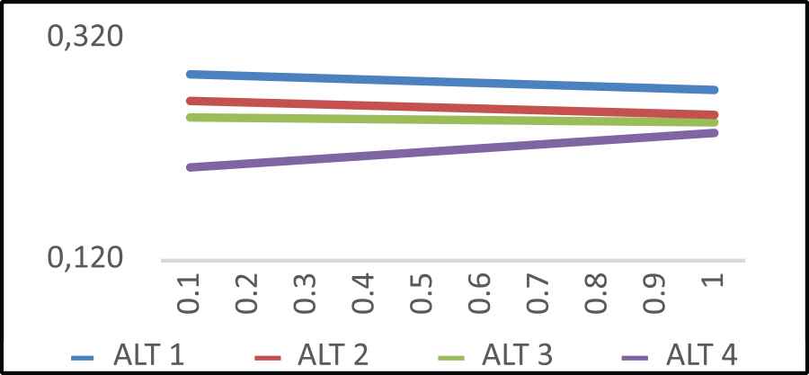
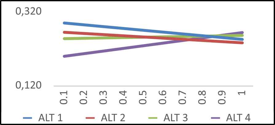
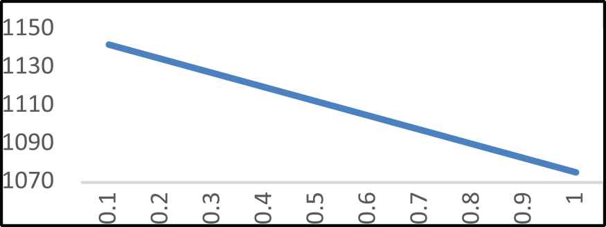
A sensitivity analysis is applied to examine the effects of the possible changes in the weights of the attributes on order prediction methodology for VMI system. Figures 2 and 3 display two results of the analysis. In these figures, the X-axis represents the weights of attributes and the Y-axis represents the possibilities of alternatives. In this analysis, the value of attributes’ weights is changed while other attribute weights are proportionally distributed. For instance, when the Location’s (A1) weights have changed from 0.138 to 0.100, the weight of Experience Level (A2) is updated as
Sensitivity analysis of attribute location (A1).
Sensitivity analysis of attribute promotional activities (A4).
This process is conducted for all attributes, and new attribute weights and alternative scores are calculated. Sensitivity analysis represents that all the attributes except Promotional Activities (A4) have no sensitivity on the ranking of alternative possibilities. But when the weight of A4 has passed 0.90, the ranking of alternative options are changing. This result approves our weights that the previous section found, which is the essential attribute is Promotional Activities (A4). It also means that decisions for the retailer are robust against the possible changes in attribute weights. In Figures 4 and 5, we can see the final scores changes according to different weights of attributes. Location (A1), Experience Level (A2), Competitors’ Activities (A3), and Promotional Activities (A4) have a positive impact while Financial Stability (A5), Current Stock (A6), Customer Order (A7), and Physical Capacity (A8) have negative consequences. It is also seen that while the weight of the most critical attribute, Promotional Activities (A4), are increasing, it affects the results more than others that total score has passed High Surplus (ALT3) level.
Sensitivity analysis results of retailer (location).
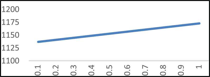
Sensitivity analysis results of retailer (financial stability).
6.3. Comparison Results
In the proposed methodology, three equal decision-makers from different FMCG company teams have evaluated the retailer based on given attributes.
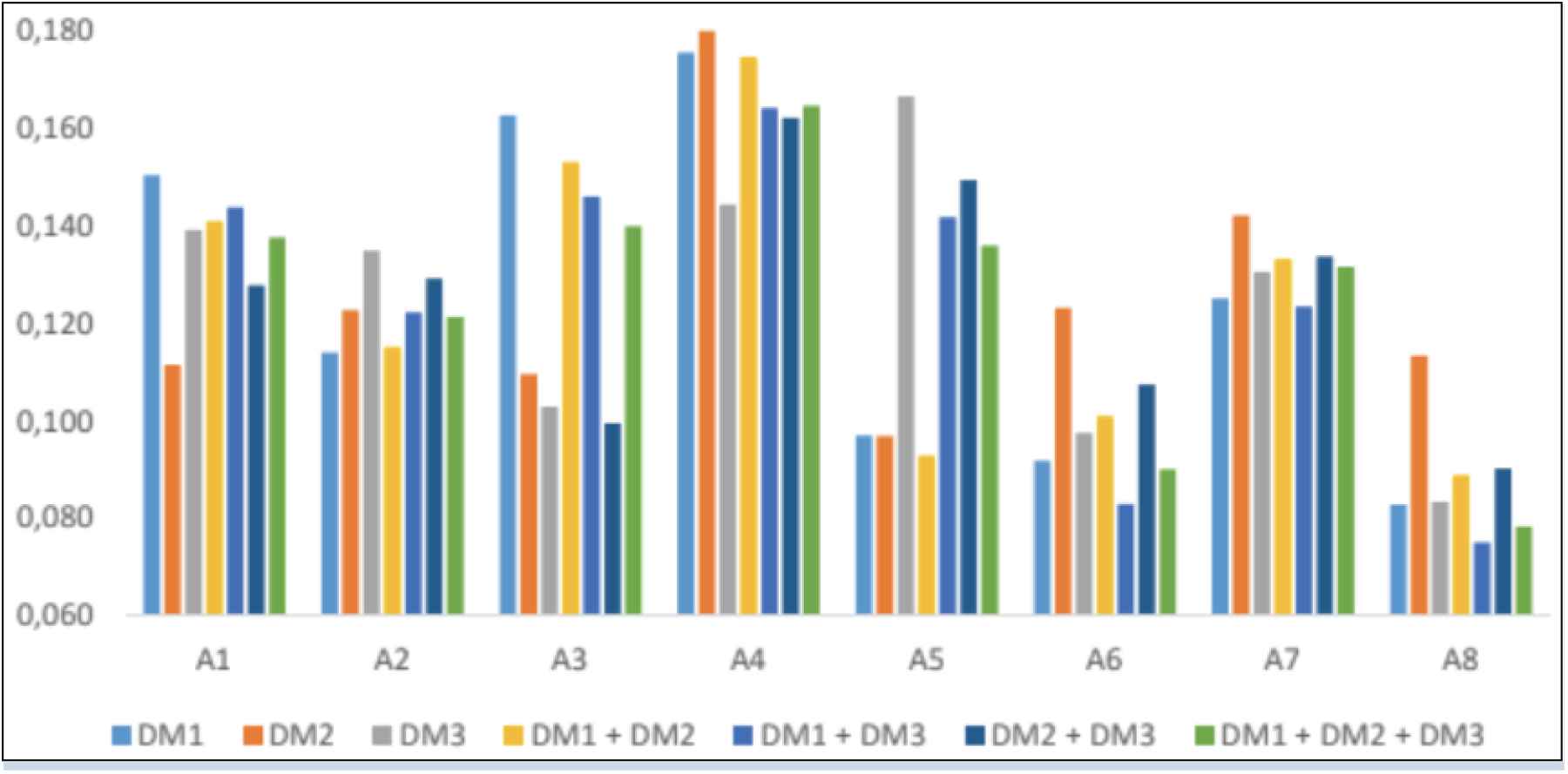
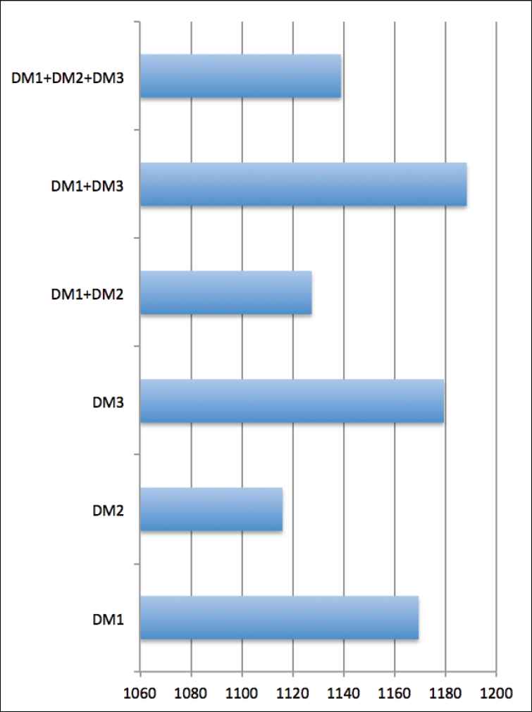
We have found that the collaboration of DM1 and DM3 has the highest value, please refer to Figure 6.
Attribute weights with respect to decision-makers’ preference.
This result shows that different decision-makers are essential for stable results. Otherwise, the results may be tricky for demand forecasting. It may also cause overstock or lack of inventory scenarios. Figure 7 shows the results of different combinations of decision-makers. Additionally, to observe the effects of different retailers’ conditions, the study ran for three real-life retailers with varying requirements and forecasted demand surpluses calculated from past sales data. Past sales data is synchronized for each retailer to simplify and interpret the comparison. Retailers’ information is hidden due to the sales company’s privacy conditions, and their names are R1, R2, and R3. The comparison results with linguistic evaluations for each retailer are also calculated.
Comparison of evaluations of different decision-makers.
To distinguish experts’ decisions, we have operated the model with varying decision-makers’ combinations. According to these results, although DM1 and DM3 give higher points to the retailer, DM2’s decisions are lower than others. It is also
Figure 8 summarizes the comparison results of retailers for each alternative. Comparison results show that although all the possibilities affect the total score, due to the crisp values of alternatives, possibilities of High Surplus (ALT3) and Very High Surplus (ALT4) affect the total score (DR) positively. Since R2 has the highest possibilities for these alternatives, it has the highest prediction. Although R1 has the highest and R2 has the lowest possibility for Medium Surplus (ALT2), it doesn’t affect the total score (DR) as much as the possibilities of High Surplus (ALT3) and Very High Surplus (ALT4). Thus, R2 has a higher prediction than R1. Low Surplus (ALT1) has the most insufficient effect on the total score (DR) with a crisp value of 600; it has a limited impact on the total score. Even R3 has the highest score for ALT1, and it has the lowest prediction due to the possibilities of other alternatives are lower than R1 and R2.
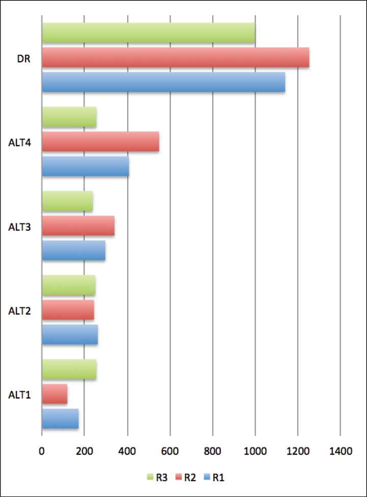
Comparison results of retailers.
7. CONCLUSION
This study concentrates on order predicting procedure, which has critical importance for a VMI system’s success. The study includes a multicriteria problem entailing to consider various quantitative and qualitative criteria for a real FMCG company. We have implemented IFSs and aggregation operators to deal with vagueness and subjectivity in human judgments.
Eight attributes that directly affect demand forecasting are considered in this study: (i) location, (ii) experience level, (iii) competitors’ activities, (iv) promotional activities, (v) financial stability, (vi) current stock, (vii) customer order, and (viii) physical capacity. They were all evaluated linguistically by three equal-weighted decision-makers from different FMCG company teams and converted to interval-valued intuitionistic fuzzy numbers. All the weights of attributes have been calculated. Promotional activities have been found as the essential attribute for demand forecasting of this FMCG company. Competitors’ activities, location, and financial stability attributes are following it. The sensitivity analysis showed that small changes in the attributes’ weight did not cause any significant changes in the end.
Additionally, for new retailer agreements, decision-makers should take the candidate’s location and financial stability into account to make a logical selection. Four alternatives have been chosen to evaluate based on eight attributes by three equally weighted decision-makers. In the proposed method, even if one of the alternatives has the highest value, the final demand surplus may be different due to the possibilities of other alternatives.
The proposed methodology avoids giving the same valuable order forecast for all retailers with different conditions and characteristics by summing the production of possibilities and demand surpluses instead of ranking the possibilities.
It is shown that experienced retailers with good location and promotion opportunities take the highest prediction while new mislocated retailers take lower forecasts.
Comparisons of different retailers showed that the proposed method yields logical and reliable results. It is also seen that the proposed order prediction methodology improves the supply chain performance of the company while preventing excessive stocks and customer backorders with equalization of the alternatives.
The comparison of the decision-makers’ results has shown that different decision-makers with different targets and characteristics are critical for stable results. Otherwise, the results may be tricky for demand forecasting.
Further studies are suggested to consider more attributes to increase the problem’s complexity, and alternatives can be increased to find more precise solutions. Additionally, other fuzzy multicriteria decision-making methods or other extensions of fuzzy sets such as hesitant fuzzy sets, type-2 fuzzy sets can also be used for the same problem.
REFERENCES
Cite this article
TY  - JOUR
AU  - Murat Levent Demircan
AU  - Ekin Merdan
PY  - 2021
DA  - 2021/04/29
TI  - A Proposed Order Prediction Methodology for Vendor-Managed Inventory System in FMCG Sector Based on Interval-Valued Intuitionistic Fuzzy Sets
JO  - International Journal of Computational Intelligence Systems
SP  - 1489
EP  - 1500
VL  - 14
IS  - 1
SN  - 1875-6883
UR  - https://doi.org/10.2991/ijcis.d.210423.004
DO  - 10.2991/ijcis.d.210423.004
ID  - Demircan2021
ER  -