
Electricity Peak Load Forecasting using CGP based Neuro Evolutionary Techniques
- DOI
- 10.1080/18756891.2016.1161365How to use a DOI?
- Keywords
- load forecasting; evolutionary algorithm; Cartesian Genetic Programming; CGPANN
- Abstract
Proficient Economic and Financial planning is critical to the successful and efficient operation of power generating and distributing units. This planning becomes quite facile if the accurate and precise knowledge regarding the required power load is ascertained. This research is an innovative effort to bring forward different electric peak load forecasting models based on the Neuroevolutionary technique known as the Cartesian Genetic Programming Evolved Artificial Neural Network(CGPANN). Although CGPANN in itself is not novel but its application to power load forecasting is quite unique because of its innate ability to identify the best computationally efficient predictive model along with the recognition of the best appropriate features for load forecasting. Both the Feedforward and Recurrent CGPANN setups have been evolved here for peak load forecasting on a daily basis. The different setups developed have been trained and tested on the peak load data of United Kingdom National Grid. The models developed in this research have been tested and compared against previously proposed machine learning models. In comparison to contemporary models in the field, a more efficient and accurate peak load forecasting model has been produced using CGPANN based prediction methods.
- Copyright
- © 2016. the authors. Co-published by Atlantis Press and Taylor & Francis
- Open Access
- This is an open access article under the CC BY-NC license (http://creativecommons.org/licences/by-nc/4.0/).
1. Introduction
Efficient and optimal utilization of electric power is directly dependent upon practical knowledge of the user consumption needs and requirements. Accurate and complete estimation of the required electricity loads is compulsory for the competent operation of a power generation unit. A number of important and critically complex issues become prevalent when an increase in the growth of power generation capacity is considered. The most important problem among these issues is the maximization of optimal performance achievement with increased operation of electric power utilities. Precise Load Forecasting has thus become necessity for the power utilities to deal with future economic growth while maintaining maximum operational efficiency. Moreover a competent load forecasting technique is not only beneficial for the suitable design of an adept power production and supply system, but also aides in the management of electric power with correct financial and monetary planning during power generation. Accurate forecasts have nowadays become crucial while planning the maintenance schedule and strategy of power generators. This also assists in making the choice for a correct combination of the available on-line capacity.
Load forecasting can be distinctively divided into three different kinds or categories. The first kind is the long term load forecasting which predicts the loads for a time frame of a year or more. The second kind is the medium term load forecasting which forecasts load for a month ahead time, and the third is the short term load forecasting which gives the load predictions on half-hourly, hourly, daily or on a weekly basis. The current research is an initiative to develop intuitive and smart systems for the short-term daily peak load forecasting using an efficient Neuroevolutionary technique known as the Cartesian Genetic Programming Evolved Artificial Neural Network(CGPANN). Neuro-Evolution is an innovative approach that leads to the artificial evolution of the entire structure as well as the components of an Artificial Neural Network(ANN). A CGPANN is a technique developed by incorporating the features of both Cartesian Genetic Programming(CGP)23 and ANNs, while using Neuroevolution to evolve the final network. The CGPANN inherits many important features of the ANN along with the quality of being Feedforward or Recurrent. The use of both the Feedforward as well as Recurrent CGPANN for short term daily peak load forecasting is quite innovative as it helps in identifying computationally efficient models. Moreover it helps in selecting the appropriate features on the basis of which the best decision regarding the required optimal load can be taken. The CGPANN based forecasters provide better accuracy than most models introduced till date as they have the flexibility of complete network parameter optimization with the best feature selection. Thus the introduction of CGPANN to the said application of load forecasting is quite noteworthy. The current research is therefore an effort to develop four different kind of forecasters using both the Feedforward as well as Recurrent CGPANN models. A comparison of the models proposed here with previously short term peak load forecasters greatly highlights the superior performance of the CGPANN models over previously proposed methodologies.
2. Literature Review
2.1. Electric Power Load Forecasting
Forecasting has been addressed in many different ways in literature. Mostly the techniques discussed involve financial and power load forecasting. Forecasting has also been applied to stock exchange in order to predict the future currency trends. Harrald and Kamstra35 have evolved Artificial Neural Networks(ANNs) to combine the financial forecasts. They compared the evolved ANNs against various linear methods with ANN models giving a superior performance as compared to the linear forecasting models like Least Mean Square Method. Wagner et al.36 have developed a Dynamic forecasting genetic programming model for time series prediction and have tested the forecasting efficiency using both real-time and simulated data. The choice of fitness measure plays a significant role in their forecasting model. Yu et al.37 have used Genetic Programming to produce a Least Square Support Vector Machine(LSSVM) for predicting stock market trends. The LSSVM input features during learning are selected by a Genetic Algorithm. The developed model outperforms many of the previously proposed forecasting models in terms of hit ratio. Huang et al.14 have developed a Hierarchical Coevolutionary Fuzzy Predictive Model(HiCEFS) for forecasting financial time series. The developed model uses a careful strategy for trading on the basis of Percentage Price Oscillator(PPO).
Nogales et al.38 have used time series analysis tools, namely dynamic regression and transfer function models for prediction of electricity prices for the next day. Both techniques have been compared against each other on real world case data of Spanish and Californian Markets. The developed models give 3–5% prediction error. Conejo et al.39 proposed a day ahead electricity price forecasting model using wavelet transform and Autoregressive Integrated Moving Average (ARIMA) model. The model has been tested on the real time pricing data of main land Spain within the year 2002 producing competitive performance.
Kalman filtering based load forecasting are one of the oldest predictive techniques utilized for power load forecasting. One of the most common form of Kalman filtering based predictive technique is the Phase Locked Loop filter1. It utilizes pattern recognition techniques along with weather patterns to predict hourly electric load. Zhang et al.2 used a hybrid technique based on the combination of Kalman filter and wavelets to develop two models for prediction of load on hourly basis. One of these models is weather sensitive and the other insensitive. Another hybrid technique involving a combination of the Kalman Filter along with Elman Neural Network was proposed in3. It uses Kalman filter to predict the linear parameters and Elman Neural Network the non-linear parameters.
Al-Hamadi and Soliman4 utilized a technique based on the hybridization of the Kalman Filter and Fuzzy logic to predict the short term peak load based on the current weather patterns as well as the recent past history. Multiple regression based techniques utilizing more than one parameter can also be utilized for load forecasting. A short term load forecasting model has been proposed by Charytoniuk et al.5 using a non parametric regression model. It was beneficial and uncomplicated, since it required easily calculated small number of parameters. Papalexopoulos and Hesterberg6 developed a new kind of hourly load forecasting model using regression models which initially predicted the maximum daily load and then this value was used to predict peak load on an hourly basis. Hagan and Behr16 used time series analysis application methods for load forecasting. They used the Box-Jenkins ARMA model. The average mean error obtained by them was 3.37%.
One of the traditional approaches employed for load forecasting is the exponential smoothing. It can either be used for time series smoothing or directly for load forecasting. Christiaanse8 proposes a predictive model based on General Exponential Smoothing (GES). Training of the system is performed on hourly data and the developed model predicts peak load based on a lead time range of 1 to 24 hours. A short term load forecasting prediction model has been proposed by El-Keib et al.12based on Adaptive General Exponential Smoothing (AGES). AGES in the proposed system has been combined with power spectrum analysis for development of a forecasting model that is quite adaptable and robust. Infield and Hill13 have introduced optimal smoothing based on a trend removal technique for the prediction of load on a short term basis. The proposed model reduced the root mean square error RMSE for forecasting by 12%. Jong-Hun Lim9 developed an improved short-term load forecasting algorithm for an arbitrary education institute for fluctuations in the daily, weekly, and yearly load patterns. He analyzed and correlated it with temperature trends during the respective periods. An optimal exponential smoothing coefficient according to the selected period was used for the building load forecasts. The estimated optimal exponential smoothing coefficient derived for each selected period was then compared with past load patterns. The proposed algorithm was verified by simulation of the electric demands showing that the forecasting accuracy of the proposed algorithm is improved comparing with traditional exponential smoothing analysis having a MAPE value of 3.61%.
Ramos et al.11 developed a load forecasting method for short-term load forecasting (STLF), based on Holt-Winters exponential smoothing and an artificial neural network (ANN). His main contributions was the application of Holt-Winters exponential smoothing approach to the forecasting problem and, as an evaluation of the past work, data mining techniques were also applied to short-term Load forecasting. Both ANN and Holt-Winters exponential smoothing approaches were compared and evaluated obtaining a MAPE of 7.6% being the best performance.
Support Vector Machine (SVM) based supervised learning methods have also been employed for Daily Load Forecasting. Chen et al.17 developed an SVM based model for daily peak load estimation based on a lead time of 31 days. The error recorded for the proposed model was within 2–3%. Pai and Hong18 introduced a load forecasting model that was a combination of the Genetic Algorithm (GA) and Recurrent SVMs (RSVMG). The GA in the model predicted the free parameters of the SVM. The proposed model was claimed to produce better results than SVMs, Artificial Neural Networks (ANNs) and regression models.
Artificial Neural Networks(ANN) based load forecasting is one of the most popular techniques for load forecasting. Peng et al.19 developed an ANN model for load forecasting in which they incorporated the effect of holidays and ”sudden environmental changes” factor. S.T Chen et al.20 developed an ANN based forecasting model for 24 hours of a day with a lead time of 168 hours. Their model forecasted the weather sensitive load only. It was claimed to perform better than most of the ANN based forecasting models. Bakirtzis et al.21 proposed a Bayesian Combined Predictor (BCP) having ANN based estimators with regression predictors for short term load forecasting. The average error obtained with BCP was estimated to be 2.07%.
Hong et al.7 proposed three key elements of long term load forecasting: predictive modeling, scenario analysis, and weather normalization. The predictive models attained high accuracy from hourly data, in comparison to classical methods of forecasting using monthly or annual peak data. Further development of probabilistic forecasts through cross scenario analysis has enhanced the results. They have achieved an accuracy of 4.2% on average.
Panday et al.10 proposed procuring of Power through energy exchange based on forecasting of day-ahead load demand. There work discussed the role of ANN in day-ahead hourly forecast of the power system load in Uttar Pradesh power corporation India ltd(UPPL) so as to minimize the error in demand forecasting. A new artificial neural network (ANN) has been designed to compute the forecasted load of UPPCL. The data used in the modeling of ANN are hourly historical electricity load data. The ANN model is trained on hourly data from UPPCL from April, 2014 to June, 2014 and tested on out-of-sample data of two weeks. Simulation results obtained have shown that a day-ahead hourly forecast of load using proposed ANN was very accurate having an average MAPE of 3.05%.
Sahay et al.15 designed a new artificial neural network (ANN) to compute the forecasted load. The data used in the modeling of ANN were hourly historical data of the temperature and electricity load. The ANN model was trained on hourly data from Ontario Electricity Market from 2007 to 2011 and tested on out-of-sample data from 2012. Simulation results obtained have shown that day-ahead hourly forecasts of load using proposed ANN generated an average MAPE of 2.05% with temperature and 2.23% without temperature.
Chen et al.29 proposed a two-stage identification and restoration method to detect the typical patterns of inaccurate measurement and abnormal disturbance based on statistical criteria independent with normal distribution in first stage and Historical trend in second stage using frequency domain decomposition. The deviations of the data measurements from the typical daily curve obey normal distribution and were used as criteria in the second stage. The effectiveness of the proposed methodology has been confirmed by examples in real bus load forecasting systems obtaining a MAPE of 1.8%.
This section highlighted various load forecasting models introduced in the field, and indicated there performance in terms of MAPE values. These models are also tabulated in Table .3, 4 for comparison with the proposed models. The next section will provide a detailed overview of Cartesian Genetic Programming(CGP) the genetic programming method used in this work for evolution of Neural Networks.
2.2. Cartesian Genetic Programming (CGP)
Cartesian Genetic Programming developed by Miller and Thompson23 is a kind of genetic programming originally introduced for the evolution of feed forward digital circuits. CGP is composed of nodes or genes that make up a genotype. The genotype is a 2D grid having rows and columns. Every gene or node within this grid has inputs and a function operating on the inputs. Each node produces an output, which can then be fed as inputs to the nodes of the next columns. A CGP genotype also called a chromosome is represented as a stream of bits or integers giving information regarding each node connectivity and functions. The phenotype representation is the directed graph which shows the connectivity of the system inputs via the nodes to the system’s outputs. The fitness of each genotype determines its selection as a parent for future generation. It also determines whether the parent should be mutated to populate the next generation of offspring or should be selected as the best evolved solution. The mutation in CGP is via a single parent only. Mutation of parent involves either the mutation of an entire node, its inputs or node functions. During evolution such nodes may arise whose outputs are neither connected to the inputs of the following nodes or to system outputs. These are the junk nodes. This gives a very unique property of CGP that each and every node in CGP might not be contributing to the over-all evolved circuitry. CGP has been used to develop many efficient applications30,31,32.
2.3. Neuro-Evolution
Neuro Evolution is a phenomenon which leads to the artificial evolution of Neural Networks. Such process leads to the complete component-wise evolution of a Neural Network framework as it embodies a change in the system inputs, outputs, neuron functions, neuron’s input, weights and the complete network topology. Evolution of a specific single parameter like neuron functions, while keeping all other components fixed limits the search space leading to an ineffective solution24. Gomez et al. propose the creation of a genotype that represents the entire network solution by using Conventional Neural Evolution (CNE)25. An obvious advantage of their proposed method is that rather than evolving the chromosomes at the Neural level, it evolves them at the network level. This results in a possibly global solution. Symbiotic Adaptive Neural Evolution (SANE)26 proposed by Moriarty has the ability to evolve network topology along with the neural population. Gomez et. al have proposed an extension to SANE by the name of Enforced Sub-Population (ESP)25, having the capability to evolve a subpopulation of hidden layer neurons. Polani and Miikkulainen has proposed an extension to SANE known as Eugenic SANE (EuSANE)48 having reinforced learning as its base concept.
Stanley and Miikkulainen have presented Neuro Evolution of Augmented Topologies(NEAT) resolving the issues of gene tracking by including historical marking, using speciation to retain innovation and lead to the formation of a complex network while starting at a simple one49. Stanley later presented a real time NEAT(rtNEAT) performing real time Neuro evolution28. Reisinger et al. then presented modular NEAT, which divided the large search space into sub parts for finding solution to a complex problem50.
3. Cartesian Genetic Programming evolved Artificial Neural Network (CGPANN)
The methodology proposed for the purpose of peak load forecasting involves the use of Cartesian Genetic Programming evolved Artificial Neural Networks(CGPANN)33,34. Proven to be an efficient Neuro-Evolutionary technique, CGPANN has the strength to artificially evolve all the parameters of an Artificial Neural Network(ANN). The evolution with the CGPANN algorithm is a continuous process, which is halted only if a reasonably accurate solution is reached.
The CGPANN inherits key characteristics of a conventional Artificial Neural Network(ANN) i.e system inputs, nodes/neurons, node’s inputs, connection weights, activation functions within the node, node’s outputs and system outputs. It also inherits the ANNs mode of operations i.e. the CGPANN can also operate in a Feedforward or Recurrent mode like an ANN. As the name implies a Feed-forward CGPANN (FCGPANN) does not have any recurrent nodes as input to the network. While on the other hand a Recurrent CGPANN (RCGPANN) along with the system inputs also has feedback or recurrent nodes as input to the network. A conventional node/neuron within an FCGPANN takes in as input the outputs of preceding nodes or system inputs, multiplies these with a certain weight lying in the range [−1, 1] and sums up the weighted inputs. An activation function finally operates on the weighted sums to produce the node output. A simple node within the RCGPANN behaves in the same manner, however it can also take in as input the output from a recurrent node. A recurrent node within an RCGPANN operates by taking in as input all the main system outputs and the rest of it’s functionality remains the same as that of a conventional/simple node. The number of recurrent nodes in a RCGPANN are decided upon by setting a feedback rate. In the current research both the FCGPANN and the RCGPANN algorithms are demonstrated using the peak load data of ten previous days to predict the peak load of the eleventh day. The future populations produced during evolution of FCGPANN and RCGPANN employ the 1+λ (one parent with λ offspring) strategy23. The connections within the FCGPANN or RCGPANN are decided upon during evolution. At different evolutionary stages, such networks may arise in which the outputs from the simple nodes are not being utilized as inputs to the following nodes or being connected to the system outputs. Such nodes are termed as junk nodes or redundant nodes. These nodes may or may not become operational in future network evolutions. A node within the FCGPANN is shown in Fig. 1. The figure shows that the inputs to the nodes are represented by I1or2 and are multiplied by the weights W1or2. The function F operates on weighted sum of these inputs to produce the output O. A simple node within an RCGPANN is the same as the one shown in Fig. 1 and the difference between a simple and a recurrent node in an RCGPANN can be seen from Fig. 3. The recurrent node takes in as input the system outputs, while a simple node within the RCGPANN can take input from system inputs, preceding node inputs or recurrent node outputs.
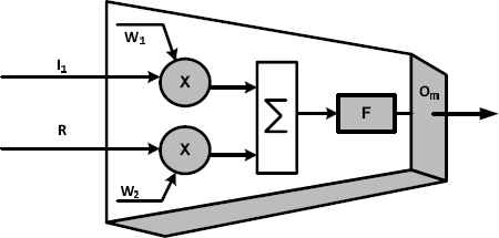
A Simple Neuron within the FCGPANN
The genotype in an FCGPANN or an RCGPANN gives a coded algorithmic representation of the network, that is then evolved to a phenotype which gives the structural representation of the same network. The genotype and phenotype representation of an FCGPANN and RCGPANN can be viewed from Fig. 2 and Fig. 4. From Fig. 2(a), it can be seen that all the columns except the last one represent the nodes within the genotype and the last column gives the connectivity of the system outputs. The node is represented by node inputs with their respective weights followed by the activation function. Fig. 2(b) represents the phenotype inferred from the genotype of Fig. 2(a). In Fig. 2(a) the column with grey color and in Fig. 2(b) the neuron within the dotted boundary are representations of junk nodes. For the RCGPANN genotype in Fig. 4(a), the first column shows that the 2nd output of the system is being fed back to the system and is being utilized as an input to the first node. Fig. 4(b) shows the phenotype representation of the genotype specified in Fig. 4(a). Junk nodes also exist in an RCGPANN, as can be viewed from the gray color column (genotype) and the dotted boundary gene (phenotype) of Fig. 4. Recurrent junk Neurons also exist in an RCGPANN. In fact there may arise a system during evolution where all recurrent neurons/nodes are redundant.
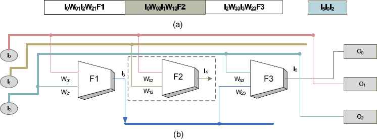
(a) Genotype (b) Phenotype Representation of FCGPANN
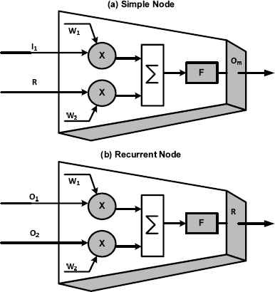
(a) A Simple Neuron within an RCGPANN (b) A Recurrent Node/Recurrent Neuron within an RCGPANN
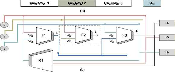
(a) Genotype (b) Phenotype Representation of RCGPANN
3.1. FCGPANN and RCGPANN Algorithm
The FCGPANN and RCGPANN algorithm can be explained from the following scheme of implementation.
- i
START
- •
INPUTS
- (a)
Nnode: Total number of neurons in a genotype.
- (b)
SInput = [i1, i2, ......, ik]: System Inputs Vector. Where k = 1, 2, ..., K, with K being the total number of system inputs.
- (c)
Ngeno: Total number of genotypes produced within a single evolutionary run.
- (d)
actF = [af1, af2, ......, afp]: Chromosome activation function list. Where p = 1, 2, ..., P, with P being the number of activation functions in the list. Here only logsigmoid is used as activation function, since it’s output is in the range of 0 and 1. The input data is also normalized in the same range. Logsigmoid function is given by the following expression:
- (e)
Inode: Total number of neuron inputs.
- (f)
μ%: Mutation rate.
- (g)
fitthresh: A fitness threshold value for stopping evolution process.
- (h)
Rμ%: Feedback rate (input for RCGPANN only).
- (a)
- •
OUTPUTS
- (a)
System Output Vector Array SOV = [op1, op2, ....., opl ], where l = 1, 2, ...., L, with L being the total number of system outputs.
- (b)
System Recurrent Nodes SRecurr (output for RCGPANN only).
- (a)
- •
- ii
INITIAL Populate Ngeno genotypes by using a pseudo random number generator51. Initialize the Ineu inputs of Nneu neurons of all Ngeno genotypes using Equation. 1 in FCGPANN and using Equation. 3 in RCGPANN. In both the equations, δ is the index of input being initialized (δ = 1, 2, ... Ineu), ζ is the index of the node whose input is being initialized (zeta = 1, 2, ...., Nneu) and χ is the genotype whose node’s input is being initialized (χ = 1, 2, ...., Ngeno). The inputs in the FCGPANN are randomly assigned either the outputs of the preceding nodes or the values from system input vector SInput, while in the RCGPANN, in addition to the preceding nodes and values from SInput, output of System Recurrent Nodes SRecurr can also be assigned.
Initialize the activation function of the Nnode neurons of Ngeno genotypes using equation 2. This equation randomly assigns an activation function from the list of activation functions actF = [af1, af2, ......, afp].Initialize the activation function of the Nnode neurons of Ngeno genotypes using equation 4. This equation randomly assigns an activation function from the list of activation functions actF = [af1, af2, ......, afp].For each χ genotype initialize the system outputs (equation 5) by forming a connection of the system output with either a system input or with a neuron output. These connections are formed by using pseudo random number generator. - iii
FITTEST GENOTYPE SELECTION From a total Ngeno genotypes, select the genotype that produces the least Mean Absolute Percentage Error(MAPE)40 in a single evolutionary iteration. This genotype is selected as a parent for the next generation. If a parent and child from the current generation have identical minimum MAPE, then choose the child as the new parent23. The same minimum MAPE used for parent selection is also compared against fitthresh and if the MAPE value is less than the threshold then the selected parent is chosen as the best evolved system followed by the termination of evolution process. If the best evolved system is not produced then the parent is mutated in step iv to continue evolution towards the best system.
- iv
MUTATION The genotype selected in the preceding step is mutated by μ % to produce Ngeno − 1 offspring. Mutation can be performed by modifying any of its characteristics (i.e neuron inputs, connection weights, activation functions, genotype output connections) selected via a pseudo random number generator. These cataleptics are mutated using equations 1, 2, 3, 4 and 5. After mutation return to step. iii for fitness evaluation of the Ngeno genotypes (Parent and Offspring).
- v
END
4. Simulation Setup
Four independent experiments are performed for generating separate prediction models to forecast the daily peak loads. One of the experiment is performed using the FCGPANN, and the other three experiments are performed to evolve RCGPANN setups with different feedback rates.
4.1. Setup 1: FCGPANN
The FCGPANN setup(see Fig. 5) evolved for daily peak load forecasting takes in as inputs the peak load data of past ten days to predict the peak load of the next calender day. For the training and system testing hourly load data has been obtained from the United Kingdom National Grid∗, which operates under extremely variant weather patterns, thus resulting in frequently varying daily peak loads. From this data the daily required peak load has been extracted. The input data is normalized between 0 and 1 in order to synchronize it with the neuron output being in the same range. The FCGPANN model has been trained on the daily peak load data of the complete year 2006 while the testing has been performed and evaluated against the daily peak load data of the years 2007, 2008 and 2009. The system has been trained to take in as input peak loads of past ten days and compute the maximum load for the next day. For the evolution of the FCGPANN, the 1 + λ approach specified for FCGPANN algorithm34 is utilized. Where λ is taken as 9 since sufficiently optimal results have been observed for this value34. Initially a random population of ten genotypes is produced. The mutation rate is set at 10%. Training and testing has been performed by changing the size of the FCGPANN, i.e. by varying the total number of nodes in the network from 50 to 500, every time with an increment of 50. The total number of inputs per node are set at 5. The FCGPANN networks produce 10 outputs which are then averaged for the final forecast value. During the training phase, the experiments on the different sized FCGPANN setups were performed for a total of two million generations each.
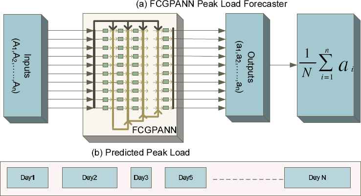
(a) FCGPANN Peak Forecasting Setup (b) Forecasted Peak Loads
4.2. Setup 2: RCGPANN with 10% Feedback Paths
The next experimental setup is that of a RCGPANN setup (see Fig. 6) having a single recurrent node (i.e. 10% feedback paths). The testing and training of the RCGPANN is done using the same data scenarios as were taken in the case of the FCGPANN setups. Evolutionary strategy of 1 + λ as specified in Section. 4.1 is used here. The major difference in this setup and that of FCGPANN of Section. 4.1 is that a recurrent node has been added to the genotypes during evolution.
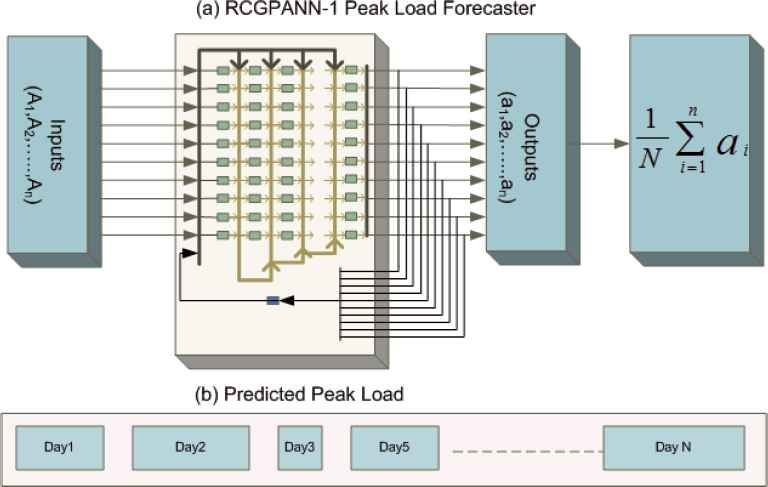
(a) RCGPANN-1 Peak Forecasting Setup (b) Forecasted Peak Loads
4.3. Setup 3: RCGPANN with 50% Feedback Paths
This setup is practically the same as the previously discussed RCGPANN setup. The only difference lies in the feedback paths, which have now been changed to 50% i.e. 5 recurrent nodes, rather than a single recurrent node as was the case with the setup in Section. 4.2. Fig. 7 shows the RCGPANN setup with 50% feedback paths.
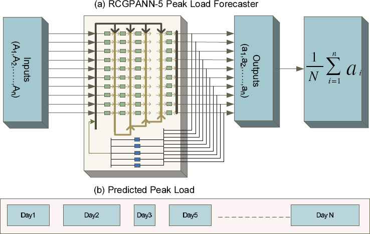
(a) RCGPANN-5 Peak Forecasting Setup (b) Forecasted Peak Loads
4.4. Setup 4: RCGPANN with 100% Feedback Paths
This setup has 10 recurrent nodes as feedback inputs during evolution. All other characteristic of the setup remain the same as the ones specified in Sections. 4.2 and 4.3. The RCGPANN setup with 10 feedbacks can be seen from Fig. 8.
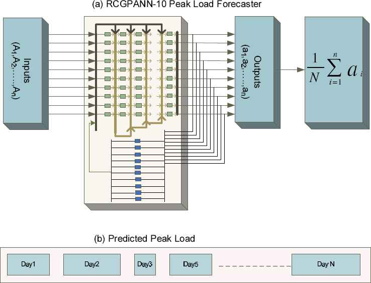
(a) RCGPANN-10 Peak Forecasting Setup (b) Forecasted Peak Loads
5. Simulations and Results
Training and testing of the Load forecasting setups has been carried out on a seasonal as well as on yearly basis. For training the data of year 2006 has been utilized, while the testing has been carried out against the data obtained for the years 2007, 2008 and 2009. For training the Root Mean Square Error (RMSE) was utilized for fitness evaluation, while MAPE, Mean Square Error (MSE) and Root Mean Square Error (RMSE) were used for performance evaluation during testing of the setups. The training error for the four types of setups with varying number of nodes can be seen from Table. 1. From the table it can be seen that the minimum RMSE obtained for the FCGPANN steup training is for a total of 350 nodes scenarios. For the RCGPANN setup with single feedback, the best RMSE is obtained for the setup with 250 nodes, while for RCGPANN setups with 5% and 10% feedback paths give the best RMSE with 100 and 250 total nodes respectively.
| Model | Feedback Outputs | No of Nodes |
|||||||||
|---|---|---|---|---|---|---|---|---|---|---|---|
| 50 | 100 | 150 | 200 | 250 | 300 | 350 | 400 | 450 | 500 | ||
| MAPE | 0 | 2.4540 | 2.4206 | 2.4538 | 2.4424 | 2.4271 | 2.4432 | 2.4097 | 2.5960 | 2.4208 | 2.4332 |
| 1 | 2.4392 | 2.4160 | 2.4331 | 2.4271 | 2.4108 | 2.4493 | 2.4361 | 2.4737 | 2.4525 | 2.4433 | |
| 5 | 2.4887 | 2.4153 | 2.4494 | 2.4321 | 2.4311 | 2.4539 | 2.4452 | 2.4308 | 2.4179 | 2.4472 | |
| 10 | 2.6985 | 2.6943 | 2.4538 | 2.4396 | 2.4125 | 2.4433 | 2.4540 | 2.4887 | 2.4400 | 2.4098 | |
| MSE | 0 | 0.1269 | 0.1279 | 0.1269 | 0.1302 | 0.1269 | 0.1271 | 0.1286 | 0.1465 | 0.1277 | 0.1279 |
| 1 | 0.1280 | 0.1284 | 0.1281 | 0.1281 | 0.1279 | 0.1304 | 0.1325 | 0.1288 | 0.1275 | 0.1315 | |
| 5 | 0.1276 | 0.1284 | 0.1275 | 0.1281 | 0.1272 | 0.1269 | 0.1274 | 0.1272 | 0.1279 | 0.1304 | |
| 10 | 0.1448 | 0.1486 | 0.1269 | 0.1282 | 0.1276 | 0.1271 | 0.1269 | 0.1276 | 0.1270 | 0.1286 | |
| RMSE | 0 | 2.4540 | 2.4206 | 2.4538 | 2.4424 | 2.4271 | 2.4432 | 2.4097 | 2.5960 | 2.4208 | 2.4332 |
| 1 | 2.6985 | 2.4160 | 2.4331 | 2.4271 | 2.4108 | 2.4493 | 2.4361 | 2.4737 | 2.4525 | 2.4433 | |
| 5 | 2.4887 | 2.4153 | 2.4494 | 2.4321 | 2.4311 | 2.4539 | 2.4452 | 2.4308 | 2.4179 | 2.4472 | |
| 10 | 2.4392 | 2.6943 | 2.4538 | 2.4396 | 2.4125 | 2.4433 | 2.4540 | 2.4887 | 2.4379 | 2.4098 | |
Training Values MAPE, MSE and RMSE for the four kinds of setups with different Number of Nodes
Table. 2 gives the MAPE values obtained for all the four setups during testing. The FCGPANN setup with 350 nodes gives the best annual MAPE value for the year 2008. This setup can be seen in Fig. 9. The setup only has two active nodes and calculates the peak load using the expression provided in Equation. 6. The difference between actual and estimated peak load values for the year 2008 using this setup can be seen from Fig. 10. The same setup also gives the minimum MAPE value for the winter season of year 2007. The actual versus estimated forecasts of peak load for winter 2007 with this setup can be observed from Fig. 11. The irregularities between actual and estimated forecasts lie within the period of end November and mid-December of 2007 and can be removed by further fine tuning during training. The data for this specific period can be removed and used to train another network that will serve as forecaster for that time period only. This will enhance the ability for the networks to accurately forecast the data; though will increase the computational cost having two independent networks.
| Setup | Model | Year | Nodes | MAPE(%) |
|---|---|---|---|---|
| FCGPANN | Autumn | 2009 | 150 | 1.4312 |
| Winter | 2007 | 350 | 2.6617 | |
| Spring | 2007 | 250 | 1.5617 | |
| Summer | 2008 | 250 | 2.2459 | |
| Annual | 2008 | 350 | 2.1847 | |
| RCGPANN-1 | Autumn | 2009 | 200 | 1.5597 |
| Winter | 2007 | 250 | 2.6914 | |
| Spring | 2007 | 100 | 2.5712 | |
| Summer | 2008 | 50 | 2.235 | |
| Annual | 2008 | 250 | 2.1884 | |
| RCGPANN-5 | Autumn | 2009 | 150 | 1.4652 |
| Winter | 2007 | 50 | 2.6740 | |
| Spring | 2007 | 50 | 1.6107 | |
| Summer | 2008 | 50 | 2.2486 | |
| Annual | 2008 | 100 | 2.1904 | |
| RCGPANN-10 | Autumn | 2009 | 150 | 1.4310 |
| Winter | 2007 | 500 | 2.6611 | |
| Spring | 2007 | 250 | 1.6012 | |
| Summer | 2008 | 100 | 2.3988 | |
| Annual | 2008 | 200 | 2.2058 | |
Minimum MAPE values for the FCGPANN and three RCGPANN setups
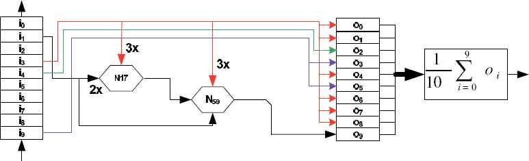
FCGPANN Setup with a total of 350 nodes
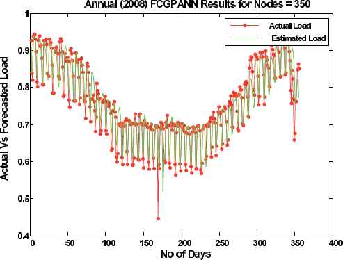
Actual Vs Forecasted 2008 Peak Load Values using FCGPANN setup of 350 Nodes.
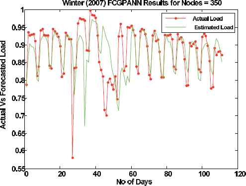
Actaul Vs Forecasted Winter 2007 Peak Load Values using FCGPANN setup of 350 Nodes.
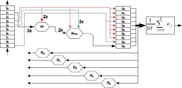
From Table. 2, it can be observed that the minimum MAPE value for the RCGPANN setup with a single recurrent node is the setup with a total of 200 nodes. The error value is obtained for peak load forecasting during Autumn 2009. The setup can be seen from Fig. 12. The evolved setup has only 4 active nodes. It can be seen from the figure that the recurrent node is also a junk node as its output is not used in the final setup obtained after all the evolutionary runs. This shows an important property of the RCGPANN that there is not a compulsion on the recurrent nodes to be used as inputs to the network. The decision regarding the use of a recurrent node as input is basically on the basis of selection during the evolutionary process. The peak load estimation for the setup in Fig. 12 is obtained from the expression given in Equation. 7 to Equation. 11. A comparison of the actual versus estimated values for the setup of Fig. 12 can be seen in Fig. 13.
200 nodes RCGPANN Setup with one feedback
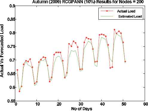
Actaul Vs Forecasted Autumn (2009) Peak Load Values using RCGPANN-1 feedback setup of 200 Nodes.
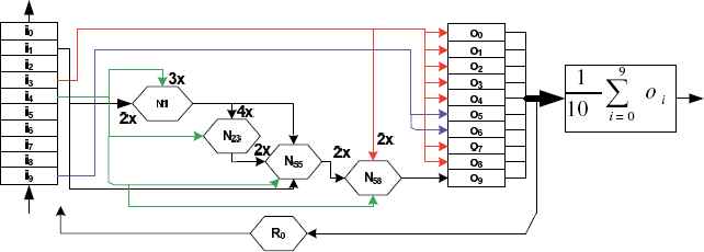
It can be further observed from Table. 2, that the RCGPANN setup with 5 recurrent node gives the minimum MAPE value for the setup with 150 nodes (see Fig. 14) during August 2009. Equation. 12 gives the expression used for peak load forecasting. The RCGPANN setup with 10 recurrent nodes also gives the minimum MAPE on the seasonal data of Autumn 2009 (see Fig 16). The minimum MAPE for the Spring and Summer seasons is obtained while forecasting values during 2007 and 2008 respectively. For the Spring 2007, the RCGPANN setup had a total of 250 nodes. The actual versus forecasted values for this setup can be observed from Fig. 15. The expression in Equation. 13 forecasts the estimated values.
150 Node RCGPANN Setup with 5 feedbacks
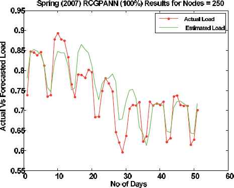
Actaul Vs Forecasted Spring 2007 Peak Load Values using RCGPANN 10 feedback setup of 250 Nodes.
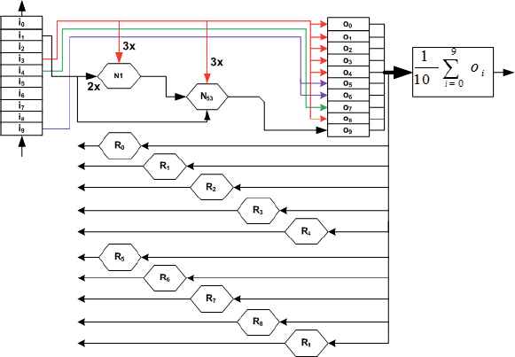
250 Node RCGPANN Setup with 10 feedbacks
A comparison of the currently proposed setups with the contemporary techniques previously introduced can be seen in Table. 3. From the table it is evident that the FCGPANN and RCGPANN are competitive in comparison to their predecessors.
| S.No | Technique | % MAPE | Testing Data | Year | No of Days | Model |
|---|---|---|---|---|---|---|
| 1 | Non-Fixed ANNs 41 | 2.45 | Hang Zhou Electric Power Company | 2001 | 30 | Summer |
| 2 | ANN based Models 10 | 3.05 | Uttar pardesh Power Corporation Ltd. | 2014 | 15 | Summer |
| 3 | Proposed Scheme with FCGPANN | 2.2459 | UK National Grid(London) | 2008 | 110 | Summer |
| 4 | Proposed Scheme with RCGPANN-1 | 2.235 | UK National Grid(London) | 2008 | 110 | Summer |
| 5 | Proposed Scheme with RCGPANN-5 | 2.2486 | UK National Grid(London) | 2008 | 110 | Summer |
| 6 | Proposed Scheme with RCGPANN-10 | 2.3988 | UK National Grid(London) | 2008 | 110 | Summer |
| 7 | Functional clustering and linear regression42 | 6.55 | Italian Grid | 2001–2002 | 198 | Annual |
| 8 | Probabilistic forecasts through cross scenario analysis by Hong et al. 7 | 4.2 | North Carolina Electric Membership Corporation (NCEMC)(USA) | 2005–2006 | 365 | Annual |
| 9 | ARIMA and GARCH 47 | 2.24 | UK National Grid(London) | 2003 | - | Annual |
| 10 | Exponential smoothing analysis by Jong-Hun Lim9 | 3.61 | Building Energy Management System (BEMS) | 2013 | 365 | Annual |
| 11 | Holt-Winters exponential smoothing and an artificial neural network (ANN) by Ramos et al. 11 | 7.60 | FEDER Funds through the Programa Operacional Factores de Competitividade COMPETE program and by National Funds through FCT Fundao para a Cilncia e a Tecnologia. | 2013 | 365 | Annual |
| 12 | ANN models by Sahay et al. 15 | 2.23 | Ontario Electricity Market | 2012 | 365 | Annual |
| 13 | Proposed Scheme with FCGPANN | 2.1847 | UK National Grid(London) | 2008 | 365 | Annual |
| 14 | Proposed Scheme with RCGPANN-1 | 2.1884 | UK National Grid(London) | 2008 | 365 | Annual |
| 15 | Proposed Scheme with RCGPANN-5 | 2.1904 | UK National Grid(London) | 2008 | 365 | Annual |
| 16 | Proposed Scheme with RCGPANN-10 | 2.2058 | UK National Grid(London) | 2008 | 365 | Annual |
MAPE comparison of FCGPANN AND RCGPANN with previous methods
Table 4 shows a similar comparison of the Mean Relative Error of RCGPANN-5 setup having a total of 50 nodes with previously proposed techniques showing that the current setup is superior in performance to its predecessors.
| S.No | Technique | % MRE | Model |
|---|---|---|---|
| 1 | Neural Networks with Weather Information 43 | 1.57 | Summer |
| 2 | Bayesian regularization, resilient and adaptive back-propagation learning based ANNs 44 | 2.43 | Summer |
| 3 | Wavelet transform and neuroevolutionary algorithm 45 | 2.02 | Summer |
| 4 | Fuzzy c means based radial basis function network 46 | 4.04 | Summer |
| 5 | Proposed Scheme with RCGPANN-5(50 nodes) | 1.5 | Summer |
Mean Relative Error comparison of FCGPANN and RCGPANN with previous methods
6. Conclusion
This work proposes the use of Neuroevolutionary Cartesian Genetic Programming evolved Artificial Neural Networks for the purpose of daily peak load forecasting of electricity loads. The evaluation of the proposed feed-forward and recurrent CGPANN networks for load forecasting is quite novel and shows very promising results. When compared against previously proposed contemporary techniques, it is observed that the current networks outperform their predecessors and give more than 98% accurate values for daily short term peak load forecasting. The incorporation of the proposed algorithms in power production and distribution units will result in a robust system with sound financial and economical use of power production resources. In future, more parameters such as weather and population growth factor can be added to improve the prediction accuracy even further.
References
Cite this article
TY  - JOUR
AU  - Gul Muhammad Khan
AU  - Rabia Arshad
PY  - 2016
DA  - 2016/04/01
TI  - Electricity Peak Load Forecasting using CGP based Neuro Evolutionary Techniques
JO  - International Journal of Computational Intelligence Systems
SP  - 376
EP  - 395
VL  - 9
IS  - 2
SN  - 1875-6883
UR  - https://doi.org/10.1080/18756891.2016.1161365
DO  - 10.1080/18756891.2016.1161365
ID  - Khan2016
ER  -