
Multi-Groups Decision Making using Intuitionistic-valued Hesitant Fuzzy Information
- DOI
- 10.1080/18756891.2016.1175812How to use a DOI?
- Keywords
- Decision making; Multi-groups decision making; Hesitant fuzzy set; Intuitionistic-valued hesitant fuzzy sets; Aggregation operator
- Abstract
Multi-groups decision making (MGDM) problems, which contain multiple groups of experts acting collectively to evaluate a set of alternatives with respect to several criteria, are focused on in this study. The existing solutions for MGDM are to aggregate the evaluations three times at different levels, which leads to less accuracy and more computational complexities. Intuitionistic-valued hesitant fuzzy elements (I-HFEs) which consider all possible values instead of aggregation straightforward are flexible to represent the experts’ opinions and lessen the steps of aggregations. This study investigates MGDM with decision information taking the form of I-HFEs and their special cases. Based on some aggregation operators of I-HFEs, three approaches for distinct scenarios of MGDM are proposed and clarified by a practical problem involved with supplier selection. Comparisons between the proposed approaches and the existing methods show that the proposed approaches are more rational than those by aggregating the evaluations directly in MGDM.
- Copyright
- © 2016. the authors. Co-published by Atlantis Press and Taylor & Francis
- Open Access
- This is an open access article under the CC BY-NC license (http://creativecommons.org/licences/by-nc/4.0/).
1. Introduction
Group decision making (GDM) is a type of participatory procedure in which multiple experts acting collectively, evaluate and select the available alternatives as a solution or solutions. Some well-known GDM methods, such as Brainstorming, 1 Delphi technique 2 and Dialectical inquiry, 3 were proposed some decades ago. According to the role of individuals, two categories of groups can be formed: heterogeneous groups and homogeneous groups. The experts in a heterogeneous group are adept at distinct fields of disciplines, and have diverse cultural backgrounds. Each expert is good at evaluating alternatives with respect to a subset of criteria. Heterogeneous group is adapted for the problems whose evaluations are interdisciplinary. The experts in a homogeneous group are from adjacent (or the same) disciplines. They have the same or similar cultural backgrounds. Each expert can conduct the same evaluation task in isolation. This kind of group is used to overcome the potential disadvantages of individuals.
In real applications, GDM is usually taken into account instead of individual decision making because of several reasons. Firstly, one expert can not afford the whole task of assessments due to the complexities of the problems. Then a group is necessary, in which each expert only needs to complete partial work. Secondly, groups own some notable advantages. It can be expected that a group takes advantage of the diverse strengths and expertise of its members, and reaches the superior solutions than the individuals. Michaelsen et al. 4 demonstrated that groups outperform their most proficient group members 97% of the time. Daily and Steiner 5 also showed that groups can achieve a higher number of brainstormed ideas.
However, there are also some disadvantages involved with GDM. It is apparent that groups are generally slower to arrive at decisions than individuals. Groupthink, sometimes, occurs when the members in the group feel pressure to confront what seems to be the dominant view of the group. Group polarization is another potential disadvantage of GDM. In addition, the members may perform the tasks quite differently. For example, individuals tend to take more risks 6 and act more selfishly 7–8 when they make decisions in a group.
In order to overcome the limitations of GDM, we present a novel decision making framework, i.e., multi-groups decision making (MGDM), to serve as a generation of traditional GDM. Generally, MGDM refers to as making decisions over available alternatives by a decision organization that is characterized by several groups. As can be seen in Part 1 of Fig. 1, the experts in each group are homogeneous while the experts in different groups are heterogeneous. Each group deals with partial evaluations according to its disciplines and backgrounds. The individuals of a group work in isolation if possible. The organization acts collectively to complete the whole work. Obviously, if there is only one group, the organization is reduced to a homogeneous group; while if there is only one member in each homogeneous group, the organization is reduced to a heterogeneous group.

The structure of multi-groups and the decision making process of a MGDM problem.
The motivation of presenting MGDM can be divided into two aspects: On the one hand, as can be seen in literature, the problems such as supplier selections, 9–10 policy-making, 11 water resource management 12 and operational risk management 13 are necessary to be conducted by multi-groups rather than a single group. On the other hand, it is interesting to combine the advantages of both heterogeneous groups and homogeneous groups by synthesizing the two categories of groups into an organization because these two categories of groups perform the tasks quite differently. Watson and Kumar 14 found that the more diverse the more conservative and the more similar the more risky. Heterogeneous groups have more problems of interaction behaviors interfered with problem-solving, whereas homogeneous groups indicate more facilitating interaction behaviors. Regarding to cultural backgrounds, culturally heterogeneous groups perform the tasks significantly better than homogeneous groups. 15 Heterogeneous groups are more likely to have unequal distributions of turns and utilize majority decisions than homogeneous groups.16 Heterogeneous groups are more effective in preventing a confirmatory information-seeking bias. 17 Moreover, the performance of homogeneous groups may be affected by ethnic culture. 16 Thus, the proper combination of these two classes of groups may alleviate their disadvantages.
Simultaneously, uncertainties are unavoidable due to the complexities of real problems. Fuzzy logic is one of the most acceptant tools to deal with both subjective and objective uncertainties. As a result, we investigate the MGDM problems in fuzzy setting. In this paper, we utilize the generalized hesitant fuzzy sets, 18 which are renamed as intuitionistic-valued hesitant fuzzy sets (I-HFSs), to study the MGDM problems with fuzzy uncertainties. Fig. 1 shows the decision making process of a single layer MGDM problem. The experts in each homogeneous group evaluate a subset of criteria of the problem and express their opinions by intuitionistic-valued hesitant fuzzy elements (I-HFEs), which can be regarded as the basic components of I-HFSs, or their special cases. The opinions obtained by one homogeneous group are synthesized by the union of I-HFEs rather than an aggregation operator. Therefore, we form the final decision matrix by all possible values instead of average values derived by some means.
Although it is not the first time of investigating MGDM, but there are some differences. Firstly, we reduce the use of aggregation operator. It is useful to deal with all the possible original values instead of considering just an aggregation operator. 18 The proposed solution for MGDM can decrease the loss of information and the computational complexities. Secondly, I-HFSs are more powerful to model uncertainties than other similar tools including Zadeh’s fuzzy sets (Z-FSs) 19, intuitionistic fuzzy sets (IFSs) 20, typical hesitant fuzzy sets (T-HFSs) 21–23, because they combine the strengths of IFSs and T-HFSs. For instance, a group is authorized to evaluate the manufacturing capability of a supplier. The experts of the group may express their opinions by means of Z-FSs, IFSs and T-HFSs. Without I-HFSs, these opinions have to be aggregated. The resultant values are not convenient to model the uncertainty of the group. But we can represent this kind of uncertainty by considering all provided values with the help of I-HFSs. Finally, I-HFSs are the generalized form of Z-FSs, IFSs and T-HFSs mathematically. Thus the experts can express their preferences by several kinds of tools, i.e., Z-FSs, IFSs, T-HFSs and I-HFSs as needed. However, many studies have developed the approaches for decision making with uncertainties in only one specific setting.
The rest of this paper is organized as follows: In Section 2, we recall some preliminaries on IFSs, intuitionistic fuzzy values (IFVs), T-HFSs, I-HFSs and I-HFEs. Section 3 defines some aggregation operators for I-HFEs. Some MGDM approaches are proposed in Section 4 and clarified by supplier selection problems in Section 5. Section 6 concludes the paper.
2. From Intuitionistic Fuzzy Sets to Intuitionistic-valued Hesitant Fuzzy Sets
In this section, we will review some basic concepts used in the paper, such as IFSs, IFVs, T-HFSs, I-HFSs, and I-HFEs.
As an extension of Z-FSs, 19 IFSs introduced by Atanassov 20 have been proven to be highly efficient to deal with uncertainties and vagueness. Recently, many authors have applied IFSs to the field of decision making 24–25 and GDM. 26–28 The concept of IFSs is as follows:
Definition 1. 20
Let X be an ordinary finite non-empty set. An IFS in X is an expression A given by
where μA : X → [0,1], νA : X → [0,1] with the condition: 0 ≤ μA (x) + νA (x) ≤ 1, for all x in X.
The functions μA(x) and νA(x) denote, respectively, the degree of the membership and the degree of non-membership of the element x in the set A. The ordered pair α(x) = (μα(x),να(x)) is referred to as an intuitionistic fuzzy value (IFV), 29 where μα(x), να(x) ∈ [0,1] and μα(x) + να(x) ≤ 1. In the rest of this paper, for a certain x in X, an IFV is abbreviated as a = (μ,ν) . Some useful operations on IFVs are listed in Appendix A.
In practice, the difficulty of evaluating the membership degrees may occur because of a hesitation among several possible values, rather than a margin of error, or some possibility distribution. Torra 21 proposed the following extension, by the union of several Z-FSs:
Definition 2 21.
Given a set of N membership functions: M = {γ1,⋯,γN}, the hesitant fuzzy set (HFS) associated with M, that is hM, is defined as hM(x) = ∪γ∈M{γ(x)}.
Afterward, Xia and Xu 30 completed the original definition of HFS by including the mathematical representation of a HFS as follows:
It is clear that HFSs are conceptually the same as set-valued fuzzy sets. 31 Most of the existing contributions focus on a special case of HFSs, i.e., T-HFSs, which assume the membership of an element is a finite non-empty subset of [0, 1]. However, we may have a doubt among several possible memberships with the form of both crisp values and interval values in [0, 1]. In order to handle this kind of assessments directly, Qian et al.18 extended the concept of T-HFSs by IFSs:
Definition 3.
The intuitionistic-valued hesitant fuzzy set (I-HFS) is defined as follows:
Note that T-HFSs, IFSs and Z-FSs are special cases of I-HFS. Given each x, we denote h = hQ (x) and call it an intuitionistic-valued hesitant fuzzy element (I-HFE).
Grattan-Guiness 31 used the union and intersection defined by Zadeh for Z-FSs. However, these operations are not recovered.32 Based on the solution proposed by Torra,21 the complement, union and intersection of I-HFEs were defined by the operations of IFVs:18
Definition 4.
Given three I-HFEs: h = ∪α∈h{α}, h1 = ∪α1∈h1 {α1} and h2 = ∪α1∈h2 {α2}, respectively, then
- (1)
Complement: hc = ∪α∈h {αc};
- (2)
Union: h1 ∪ h2 = ∪α1∈h1,α2∈h2 {α1 ∪ α2};
- (3)
Intersection: h1 ∩ h2 = ∪α1∈h1,α2∈h2 {α1 ∩ α2}.
Qian et al. 19 further defined some arithmetic operations of I-HFEs:
Definition 5.
Given three I-HFEs: h = ∪α∈h {α}, h1 = ∪α1∈h1 {α1} and h2 = ∪α1∈h2 {α2}, respectively, λ > 0, then
- (1)
- (2)
- (3)
h1 ⊕ h2 = ∪α1∈h1,α2∈h2 {α1 ⊕ α2} ;
- (4)
h1 ⊗ h2 = ∪α1∈h1,α2∈h2 {α1 ⊗ α2}.
Arithmetic operations in Definition 5 satisfy the following distributive laws:
Theorem 1. 18
Given three I-HFEs h, h1 and h2, λ, λ1, λ2 > 0, then we have:
- (1)
(λ1 + λ2)h = λ1h ⊕ λ2h ;
- (2)
λ(h1 ⊕ h2) = λh1 ⊕ λh2.
In decision making, we usually need to distinguish preference information provided by the experts. Qian et al.18 gave some definitions to measure I-HFSs:
Definition 6.
Let α = (μα,να) be an IFV, the expect value of α is defined as E (α) = (μα + 1 − να)/2 . The score function and consistency function of a I-HFE h, denote by s(h) and c(h), respectively, is defined as:
Definition 7.
Given two I-HFEs h1 and h2, then
- (1)
if s(h1) < s(h2), then h1 is smaller than h2, denoted by h1 < h2;
- (2)
if s(h1) = s(h2), then
- a)
if c(h1) < c(h2), then h1 is smaller than h2, denoted by h1 < h2;
- b)
if c(h1) = c(h2), then h1 and h2 represent the same information, denoted by h1 = h2.
- a)
Remark 1.
Chen et al. 33 defined a similar extension of HFSs, i.e., interval-valued hesitant fuzzy sets. The elements of which take the form of intervals in [0, 1]. The main difference lies on the construction of elements. If the elements are constructed by interval-valued fuzzy numbers, then the interval-valued hesitant fuzzy sets can be used; whereas if the elements are represented by the aspects of membership and non-membership, then the I-HFSs are more suitable.
3. Information aggregation with I-HFEs
Several aggregation operators for T-HFSs have been proposed. 9, 29, 34–35 Moreover, for interval-valued hesitant fuzzy sets, Wei et al. 36 developed several arithmetical operators, geometric operators and some dependent operators. The Einstein operator can also be found in Wei and Zhao. 37 To resolve the MGDM problems mentioned in this paper, it is necessary to develop some novel arithmetic and geometric aggregation operators in the intuitionistic-valued hesitant fuzzy setting.
To facilitate the application of I-HFEs, Qian et al. 18 introduced the following extension principle to export the operators on IFVs to I-HFEs:
Definition 8.
Let Θ be a function Θ: [0,1]N → [0,1], H = {h1,h2,⋯,hN} be a set of I-HFEs on the reference set X. Then the extension of Θ on H is defined for each x in X by:
Based on Definition 8, the existing aggregation operators of IFVs can be employed to aggregate a collection of I-HFEs. To meet the application in Section 4, we specify some aggregation operators of I-HFEs in this section.
3.1. Some operators for aggregating I-HFEs
When aggregating a collection of numerical information associated with their weights, one of the most straightforward ways is the weighted averaging. Xu 29 developed the intuitionistic fuzzy weighted averaging (IFWA) operator by extending the weighted averaging operator. 38 Moreover, the generalized aggregation operators 39–40 were proposed by the idea of the generalized mean operator. 41 Zhao et al. 39 presented the generalized aggregation operators for IFVs. Based on which, we develop the following generalized aggregation operators of I-HFEs based on the extension principle:
Definition 9.
Let hj (j = 1,2,⋯,n) be a set of I-HFEs, w = (w1,w2,⋯,wn)T be the weight vector of them such that
Let’s consider some special cases of the GIHFWA operator obtained by the distinct mechanisms of w and λ.
If λ = 1, then the GIHFWA operator is reduced to the IHFWA operator:
If λ → +∞, then the GIHFWA operator is reduced to the maximum operator of I-HFEs:
If λ = 1 and w = (1/n, 1/n,⋯,1/n)T, then the GIHFWA operator is reduced to the intuitionistic-valued hesitant fuzzy arithmetical averaging (IHFAA) operator.
Example 1.
Let h1 = {(0.5,0.4),0.65}, h2 = {(0.6, 0.2)}, h3 = {(0.4,0.55), (0.55,0.35)}, and the weighting vector w = (0.2,0.5,0.3)T. Then if λ = 1, we have
Furthermore, GIHFWA5(h1,h2,h3) = {(0.5464, 0.2769), (0.5705, 0.2596), (0.5806, 0.2720), (0.5995, 0.2553)}, GIHFWA-1(h1,h2,h3) = {(0.5203, 0.3287), (0.5654, 0.2769), (0.5510, 0.3194), (0.5955, 0.2684)}.
Despite being a simply and straightforward way to fuse information, arithmetic averaging usually suffers form extreme values. Geometric averaging, 42 services as another important mean, is influenced by extreme values much more slightly, except for 0 and negative numbers (Note that negative numbers are not emerged in this study). Furthermore, the geometric averaging is the only consistent function to aggregate the rates of increases/decreases. Thus, this averaging strategy owns wide application in economics, for instance, computing averaging level of development and predicting stock-price. 43 Xu and Yager 44 presented the intuitionistic fuzzy weighted geometric (IFWG) operator, motivated by which, we develop a similar operator of I-HFEs:
Definition 10.
Let hj (j = 1,2,⋯,n) be a set of I-HFEs, w = (w1,w2,⋯,wn)T be the weight vector of them such that
Similarly, we discuss some special cases of the GIHFWG operator obtained by the distinct w and λ.
If λ = 1, then the GIHFWG operator is reduced to the IHFWG operator:
If λ = 1 and w = (1/n, 1/n,⋯,1/n)T, then the GIHFWG operator is reduced to the intuitionistic-valued hesitant fuzzy geometric averaging (IHFGA) operator.
If λ → 0, then the GIHFWA operator is reduced to the IHFWG operator.
Example 2.
Let h1 = {(0.4,0.55),(0.55,0.35)}, h2 = {(0.7,0.2)}, h3 ={(0.5,0.4),0.9}, and the associated weighting vector w = (0.2,0.5,0.3)T. Then according to (11): if λ = 1, then IHFWG(h1,h2,h3)= {(0.5658, 0.3459), (0.6749, 0.2613), (0.6030, 0.2960), (0.7193, 0.2049)}; if λ = 2, then GIHFWG2(h1,h2,h3)= {(0.5532, 0.3671), (0.6392, 0.3018), (0.5955, 0.3068), (0.6983, 0.2199)}.
3.2. Properties of the proposed operators
Based on the definitions hereinabove, we present some properties of the operators to ensure their rationalities in decision making. In this section, a collection of I-HFEs hj(j = 1,2,⋯,n) are denoted by hj = ∪{αjij} (j = 1,2,⋯,n), where αjij = (μjij,νjij) is the ij th IFV of hj, ij = 1,2,⋯,#hj, j = 1, 2,⋯,n.
Theorem 2.
(Idempotency) Let hj (j = 1,2,⋯,n) be a set of I-HFEs, w = (w1,w2,⋯,wn)T be the weight vector of them such that
- (1)
GIHFWAλ (h1,h2,⋯,hn) = h,
- (2)
GIHFWGλ (h1,h2,⋯,hn) = h.
Proof.
See Appendix B.
Note that the condition of Theorem 2 is that all hj (i = 1,2,⋯,n) are absolutely the same. Thus if hj = h (by Definition 7), generally, this property does not always hold.
Theorem 3.
(Boundary) Let hj (j = 1,2,⋯,n) be a set of I-HFEs, w = (w1,w2,⋯,wn)T be the weight vector of them such that
Then
- (1)
(μ−, ν+) ≤ GIHFWAλ(h1,h2,⋯,hn) ≤ (μ+, ν−),
- (2)
(μ−, ν+) ≤ GIHFWGλ(h1,h2,⋯,hn) ≤ (μ+, ν−).
Proof.
See Appendix B.
In order to discuss the monotonicity, another collection of I-HFEs ḣj (j = 1,2,⋯,n) are denoted by
Theorem 4.
(Monotonicity) Let hj, ḣj (j =1,2,⋯,n) be two collections of I-HFEs, w = (w1,w2,⋯,wn)T be the weight vector of them such that
- (1)
GIHFWAλ(h1,h2,⋯,hn) ≤ GIHFWAλ(ḣ1,ḣ2,⋯,ḣn),
- (2)
GIHFWGλ(h1,h2,⋯,hn) ≤ GIHFWGλ(ḣ1,ḣ2,⋯,ḣn).
Proof.
See Appendix B.
Note that the condition of Theorem 4 is a sufficient condition of hj ≤ ḣj. In fact, if
Furthermore, in the following, we discuss the relationship between the proposed operators. Before that, a lemma should be introduced:
Lemma 1.39
Let xj > 0, λj > 0, j = 1,2,⋯,n, and
Theorem 5.
Let hj (j = 1,2,⋯,n) be a set of I-HFEs, w = (w1,w2,⋯,wn)T be the weight vector of them such that
Proof.
See Appendix B.
Similarly, we can prove the following theorems:
Theorem 6.
Let hj (j = 1,2,⋯,n) be a collection of I-HFEs, w = (w1,w2,⋯,wn)T be the weight vector of them such that
- (1)
IHFWG(h1,h2,⋯,hn) ≤ GIHFWAλ(h1,h2,⋯,hn);
- (2)
GIHFWGλ (h1,h2,⋯,hn) ≤ IHFWA(h1,h2,⋯,hn).
The proof is omitted here. Note that we have proposed two classes of operators to enable the use of I-HFEs in potential decision making problems, such as the problems discussed in the coming section. In fact, other kinds of operators in this setting can also be developed based on the recommendation of Rodríguez et al.45
4. Multi-Groups Decision Making with I-HFEs
In this section, we focus on the solutions of the MGDM problems. We first describe the problem mathematically, and then propose some approaches corresponding to the specific MGDM problems.
4.1. Mathematical description
In the MGDM problems, several groups of experts act collectively to select the most relevant alternative(s) among the available ones. Formally, this problem can be described as follows:
A decision organization is formed by L groups (denoted by Gl(l = 1,2,⋯,L)) of experts (denoted by Δ = {elm|m = 1,2,⋯,Ml, l = 1,2,⋯,L}, where elm represents the mth expert in group Gl). The experts elm (m = 1,2,⋯,Ml) in the group Gl are homogeneous, l = 1,2,⋯,L ; while the experts of different groups are heterogeneous. The relative weights of experts within a group are indifferent. The organization is authorized to evaluate a set of alternatives A = {a1,a2,⋯,aR} in terms of a set of criteria C = {c1,c2,⋯,cP}. The weight vector of criteria is w = (w1,w2,⋯,wP)T, where
4.2. Approaches for multi-groups decision making based on different scenarios
In this section, we mainly focus on the solutions of three specific MGDM problems based on different scenarios. Let’s begin with a simple example. Suppose that a company is going to select and import the most valuable product from some alternatives. Three main criteria are the production cost, marketing cost and after-sales service cost. The manager authorizes three relative departments, i.e., the producing department, the marketing department and after-sales service department, to evaluate the product. If one criterion is only evaluated by a single department (for instance, the production costs of alternatives are only focused by the producing department), we call this case the 1-to-n scenario (because more than one criterion may be assessed by the same department). Moreover, distinct departments may pay their attention on the same criterion. For example, the production cost influences the work of all departments. Thus, they will all express their opinions about the costs of alternatives. We call this case the m-to-n scenarios. We focus on the solution of these scenarios in this section.
4.2.1. The approach for the 1-to-n scenario
This scenario assumes that each criterion is evaluated by only one group, i.e., SCl1 ∩ SCl2 = Φ for any l1,l2 = 1,2,⋯,L. As seen in Fig. 2, one group evaluates alternatives with respect to one criterion or some criteria. This scenario is close to the common GDM problems. A common approach for the scenario is to aggregate the I-HFEs within each group at first, and then aggregate the averaged evaluations for each alternative. We use the union of I-HFEs to eliminate the first aggregation. The corresponding approach, namely Approach 1, is presented as follows:
- Step 1
Forming the decision matrix D = (ĉp (ar))R×P, where the satisfaction degree of ar with respect to cp, denoted by ĉp(ar), is the I-HFE constructed by
where the expert elm in (12) is from the group Gl who has contributed his/her evaluation in terms of cp. - Step 2
The choice of the aggregation operator. Associated with w, we aggregate the overall satisfaction degree of each alternative ar by one aggregation operators of I-HFEs according to the characteristics of criteria and the preferences of DMs. For example,
where r = 1,2,⋯,R. - Step 3
The choice of the best alternative(s). Rank alternatives according to information of
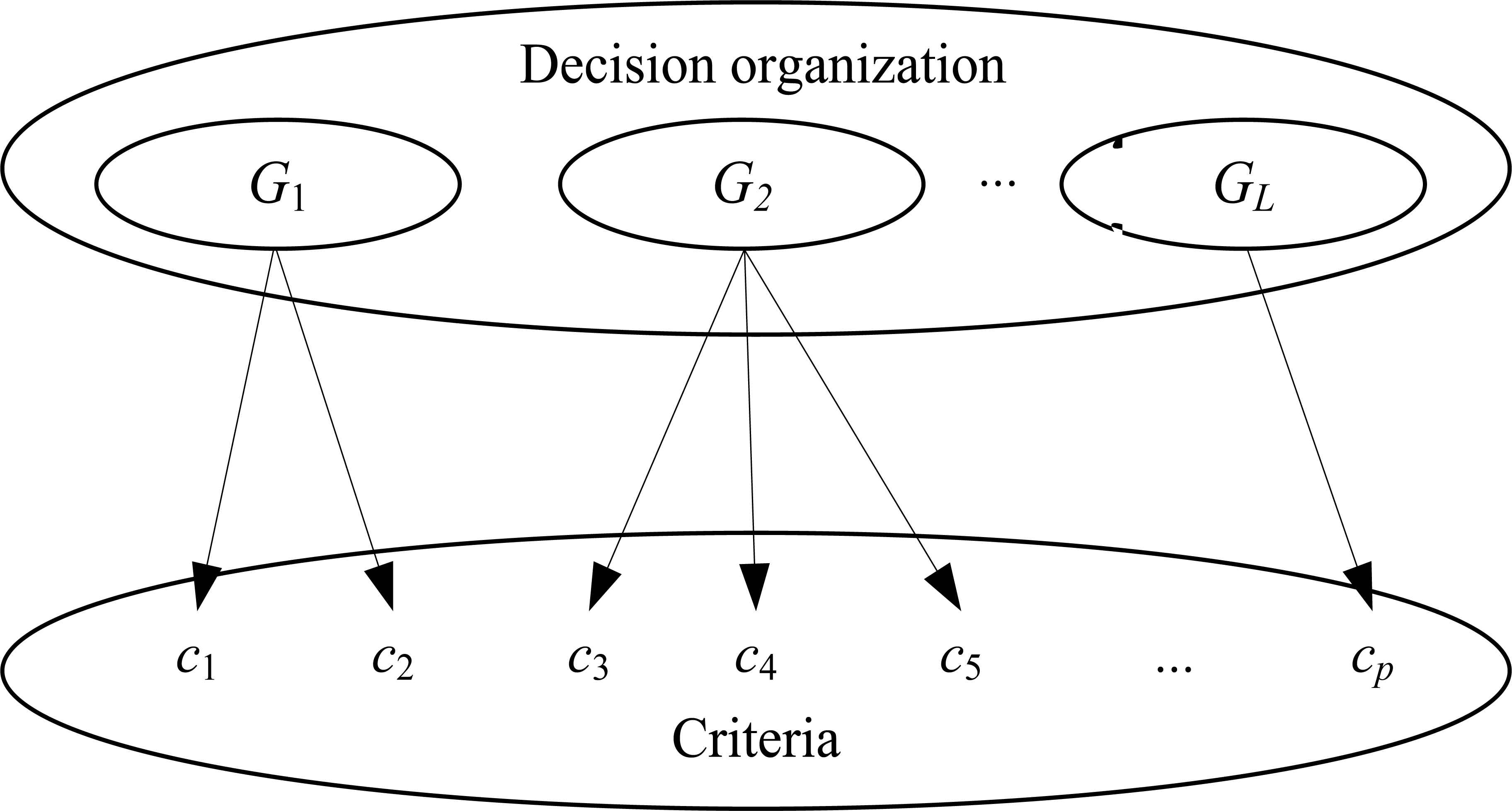
The structure of the 1-to-n scenario.
4.2.2. The approaches for the m-to-n scenario
Generally, as shown in Fig. 3, a criterion may be evaluated by more than one group. Mathematically, there may exist l1,l2 ∈ {1,2,⋯,L}, such that SCl1 ∩ SCl2 ≠ Φ. With regard to cp, the groups which participate in evaluating cp are denoted by G(p). Apparently, G(p) ⊆ G and ∪p=1,2,⋯,P G(p) = G. The experts in G(p) are denoted by
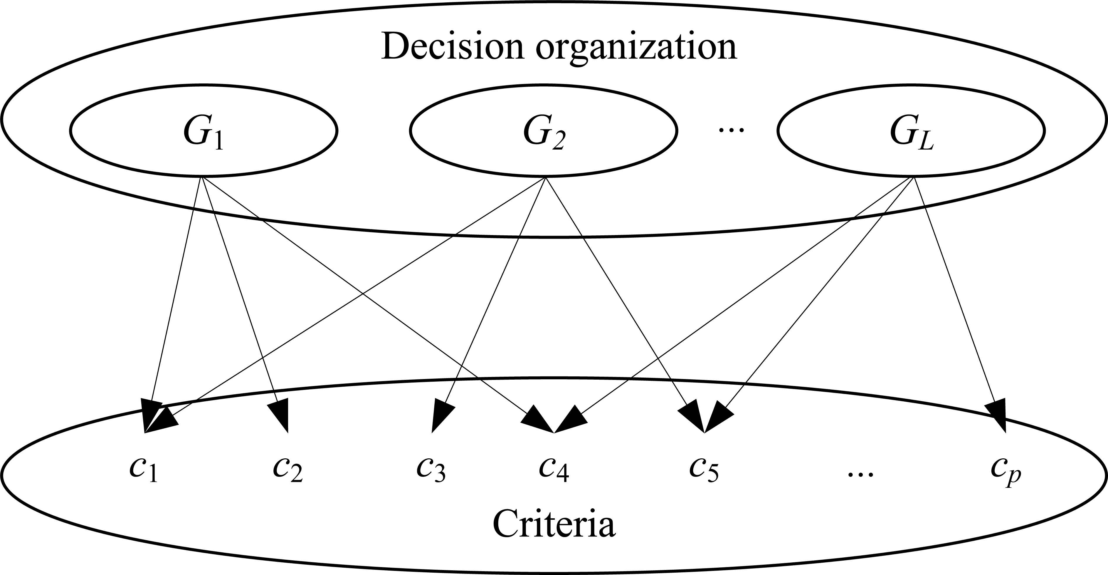
The structure of the m-to-n scenario.
Firstly, we assume that the weights of groups in G(p) are equal. In other words, they have the same confidence level when evaluating cp. A common approach of the scenario is to aggregate the I-HFEs within each group at first, then aggregate the I-HFEs within G(p), and at last aggregate the I-HFEs in the criteria level. We use the union of I-HFEs to eliminate the first two steps of aggregation. The corresponding decision making procedure, namely Approach 2, is as follows:
- Step 1
Forming the decision matrix D = (ĉp(ar))R×P. With respect to cp, ĉp(ar) is formed by the union of I-HFEs contributed by the experts
- Step 2
The choice of the aggregation operator. See Step 2 of the approach for the 1-to-n scenario.
- Step 3
The choice of the best alternative(s). See Step 3 of the approach for the 1-to-n scenario.
Secondly, we assume that the weights of groups in G(p) cannot be ignored. Generally, because of the distinguished professional area, the groups in G(p) may have different confidence levels when evaluating cp. In this case, the groups in G(p) are denoted by
- Step 1
Synthesizing evaluations within group. The satisfaction degree of ar with respect to cp, contributed by members of Gl, denoted by ĉp(ar,Gl), is synthesized by the union of I-HFEs contributed by each member:
- Step 2
Forming the decision matrix D = (ĉp(ar))R×P.
As we cannot ignore the differences of groups in G(p), ĉp(ar) is formed by a weighted aggregation operator which is used to aggregate the evaluations of the M(p) groups. For example, if the GIHFWA operator is used, then
where the weight vector - Step 3
The choice of the aggregation operator. See Step 2 of the approach for the 1-to-n scenario.
- Step 4
The choice of the best alternative(s). See Step 3 of the approach for the 1-to-n scenario.
Note that the proposed approaches eliminate one or two aggregation steps, and thus facilitate to sufficiently use the original decision information. Moreover, in the evaluation phase, the experts can express their opinions by several kinds of fuzzy sets, such as Z-FSs, IFSs, T-HFSs and I-HFSs. In order to avoid the shortages of groups, the experts are advised to work in isolation.
Generally, all the proposed aggregation operators can be used in the proposed approaches. The GIHFWA operator and the IHFWA operator own wide application areas because of the idea of arithmetical averaging. While the GIHFWG operator and the IHFWG operator are recommended to be considered if there are some extreme values (except for 0).
5. Application and Discussions
In this section, we consider a practical application involving supplier selection in a supply chain. 9–10 Then we discuss some advantages and disadvantages of the proposed approaches.
5.1. Application to a supplier selection problem
In order to reduce the risks and uncertainties of the supply chain and improve customer service, inventory levels and cycle times, the enterprise authorizes an organization, which includes 3 groups (denoted by G1,G2,G3) of experts, to select the most considerable supplier from 5 potential suppliers. The organization considers 3 aspects of criteria: (1) c1 : Performance (including delivery, quality and price); (2) c2 : Technology (including manufacturing capability, design capability and ability to cope with technology changes); (3) c3 : Organizational culture and strategy (including feeling of trust, internal and external integrations of suppliers and compatibilities across levels and functions of the buyer and supplier). The associated weight vector of these criteria is w = (0.4,0.3,0.3)T. After elementary filter, 3 suppliers a1, a2 and a3 are eligible. Thus the organization needs to evaluate these 3 suppliers using a supplier rating system. There are 2 experts in each group, denoted by elm (l = 1,2,3, m = 1,2). For the sake of convenience, the experts can express their opinion by Z-FSs, IFSs, T-HFSs and I-HFSs. After independent evaluation, all possible evaluated values provided by 6 experts are summarized in Tables 1–6.
| c1 | c2 | c3 | |
|---|---|---|---|
| a1 | {0.6} | (0.7, 0.2) | {0.4, 0.5} |
| a2 | (0.6, 0.2) | {0.5, 0.9} | {0.7} |
| a3 | (0.4, 0.5) | {0.3} | {0.6} |
The performances of alternatives with respect to 3 criteria provided by e11.
| c1 | c2 | c3 | |
|---|---|---|---|
| a1 | (0.7, 0.1) | {0.5} | {0.3} |
| a2 | {0.5} | (0.6, 0.1) | {0.5} |
| a3 | {0.6} | (0.4, 0.4) | {0.6} |
The performances of alternatives with respect to 3 criteria provided by e12.
| c1 | c2 | c3 | |
|---|---|---|---|
| a1 | {0.5} | {0.6} | {0.6} |
| a2 | {0.9} | {0.4, 0.7} | (0.6, 0.3) |
| a3 | {0.3} | (0.4, 0.5) | {0.5} |
The performances of alternatives with respect to 3 criteria provided by e21.
| c1 | c2 | c3 | |
|---|---|---|---|
| a1 | {0.4} | {0.6} | {0.4} |
| a2 | {0.7} | (0.3, 0.5) | (0.8, 0.1) |
| a3 | (0.7, 0.2) | {0.6} | (0.7, 0.1) |
The performances of alternatives with respect to 3 criteria provided by e22.
| c1 | c2 | c3 | |
|---|---|---|---|
| a1 | {0.7} | (0.4, 0.5) | {0.7} |
| a2 | {0.8} | {0.7} | {0.5} |
| a3 | {0.7} | {0.7} | {0.3} |
The performances of alternatives with respect to 3 criteria provided by e31.
| c1 | c2 | c3 | |
|---|---|---|---|
| a1 | {0.3, 0.5} | {0.4, 0.5} | {0.5, 0.6} |
| a2 | (0.5, 0.3) | (0.6, 0.2) | (0.8, 0.1) |
| a3 | {0.5} | {0.4} | {0.4, 0.5} |
The performances of alternatives with respect to 3 criteria provided by e32.
To get the optimal supplier, we follow the approaches proposed in Section 4.
- (1)
Assume that group Gi is authorized to evaluate the criterion ci according to their professional area, i = 1,2,3 . In other words, only one group is going to evaluate each criterion. Thus we use data of the first columns of Tables 1–2, the second columns of Tables 3–4 and the third columns of Tables 5–6. Following the approach for the 1-to-n scenario, we have
- Step 1
By (12), we have ĉ1(a1) = {0.6, (0.7, 0.1)}, ĉ1(a2) = {(0.6, 0.2), 0.5}, ĉ1(a3) = {(0.4, 0.5), 0.6}, ĉ2(a1) = {0.6}, ĉ2(a2) = {0.4, 0.7, (0.3, 0.5)}, ĉ2(a3) = { (0.4, 0.5), 0.6}, ĉ3(a1) = {0.5, 0.6, 0.7}, ĉ3(a2) = {0.5, (0.8, 0.1)}, ĉ3(a3) = {0.3, 0.4, 0.5}.
- Step 2
If the GIHFWG operator is used, without loss of generality, we test when λ =1, 2, 5, 10, 20. Take a1 for example, if λ =1, then the overall satisfaction degree is:
- Step 3
According to Definitions 6 and 7, the score values and the overall rankings can be seen in Table 7.
- Step 1
- (2)
Assume that each group is professional enough to undertake the whole task of evaluations, as shown in Tables 1–6, all 3 groups are going to evaluate alternatives with respect to 3 criteria. Thus it is unnecessary to distinguish with each other when synthesizing evaluations. Following Approach 2, if the GIHFWA operator is used, and λ =1, 2, 5, 10, 20, respectively, then the score values and overall rankings are shown in Table 8.
- (3)
Also assume that three groups are going to evaluate alternatives with respect to 3 criteria. If each group has a different degree of confidence when assessing with respect to different criteria, they are advised to provide a confidence level along with each provided performance (as shown in Table 9). Thus weight vectors of 3 groups of evaluating the criteria c1, c2 and c3 are w1 =(0.25,0.35,0.4)T, w2 =(0.27,0.41,0.32)T and w3 =(0.47,0.21,0.32)T, respectively. In this case, according to Approach 3, we need to aggregate the information among 3 groups and then aggregate among criteria. If the GIHFWA operator is used, and λ=1, 2, 5, 10, 20, respectively, then the score values and the overall rankings are shown in Table 10 (For each row of Table 10, for example, λ =1 means that we use the GIHFWA operator with λ = 1 wherever aggregation is needed).
|
|
|
|
Ranking | |
|---|---|---|---|---|
| λ=1 | 0.6374 | 0.5764 | 0.4790 | a1>a2>a3 |
| λ=2 | 0.6262 | 0.5598 | 0.4741 | a1>a2>a3 |
| λ=5 | 0.6096 | 0.5237 | 0.4578 | a1>a2>a3 |
| λ=10 | 0.5955 | 0.4946 | 0.4361 | a1>a2>a3 |
| λ=20 | 0.5830 | 0.4726 | 0.4153 | a1>a2>a3 |
Score values of overall performances and rankings of alternatives obtained by Approach 1.
|
|
|
|
Ranking | |
|---|---|---|---|---|
| λ=1 | 0.5460 | 0.6999 | 0.5445 | a2> a1 >a3 |
| λ=2 | 0.5530 | 0.7064 | 0.5532 | a2> a3 >a1 |
| λ=5 | 0.5731 | 0.7264 | 0.5773 | a2> a3 >a1 |
| λ=10 | 0.5959 | 0.7460 | 0.6027 | a2> a3 >a1 |
| λ=20 | 0.6165 | 0.7676 | 0.6244 | a2> a3 >a1 |
Score values of overall performances and rankings of alternatives obtained by Approach 2.
| c1 | c2 | c3 | |
|---|---|---|---|
| G1 | 0.5 | 0.6 | 0.9 |
| G2 | 0.7 | 0.9 | 0.4 |
| G3 | 0.8 | 0.7 | 0.6 |
The confidence levels of evaluating with respect to criteria provided by 3 groups.
|
|
|
|
Ranking | |
|---|---|---|---|---|
| λ=1 | 0.6040 | 0.7109 | 0.5748 | a2> a1 >a3 |
| λ=2 | 0.6064 | 0.7143 | 0.5786 | a2> a1 >a3 |
| λ=5 | 0.6279 | 0.7365 | 0.6058 | a2> a1 >a3 |
| λ=10 | 0.6596 | 0.7693 | 0.6462 | a2> a1 >a3 |
| λ=20 | 0.6946 | 0.8076 | 0.6894 | a2> a1 >a3 |
Score values of overall performances and rankings of alternatives obtained by Approach 3.
5.2. Comparing with similar techniques
According to Tables 7, 8 and 10, we can see that the ranking results are quite different. The main reasons fall into the following aspects. First, the decision information is different. For example, compared to Table 8, Table 10 is derived by the weighting groups according to the provided confident levels. Thus, it is necessary to weight groups if they are not equally professional when evaluating alternatives. In addition, as described in Section 3, the arithmetical operators and the geometric operators possess their own mathematical features. Distinct types of operators are suitable for different kinds of criteria due to their natures. Finally, if the overall performances of alternatives are close to each other, then the values of the parameter λ may result to distinct rankings, as can be seen in Table 8.
In order to compare with the existing solutions, we consider this problem by an existing method, i.e., calculating the problem with the aggregation operators in intuitionistic fuzzy setting. We need to transform all the original evaluations of Tables 1–6 into IFVs in this case. Torra 21 suggested a method to transform them by the concept of envelops. For example, {0.6, (0.7, 0.1)} is substituted by its envelop, i.e., the IFV (0.6, 0.1). Moreover, the IFWA operator 29 is used whenever the aggregation operator is needed. Table 11 shows some values emerged in the procedure of computing by using the comparable method and three proposed approaches. Furthermore, the ways to obtain these values are listed in Table 12. From the two tables, we can draw the following advantages of the proposed approaches:
- (1)
The existing method uses the averaged values at each level. While the I-HFSs based approaches keep all the possible values. For example, h(a1,c3,e32) ={0.5, 0.6} implies the expert e32 has hesitancy on 0.5 and 0.6 when evaluating a1 with respect to c1. As shown in Table 11, an IFV (0.5, 0.4), is obtained for the existing method. But the proposed approaches use the original values straightly. Therefore, when the information in the third group is synthesized, the IFV (0.6127, 0.3464) is derived by the arithmetical averaging of (0.5, 0.4) and (0.7, 0.3). But the proposed approaches consider all possible values, represented by {0.5, 0.6, 0.7}.
- (2)
The proposed approaches reduce at least one aggregation step. As clearly shown in Table 12, the existing method needs 4 aggregation steps to arrive the overall satisfactory degree of an alternative. However, the first two proposed approaches need only one aggregation step and Approach 3 need two aggregation steps. Note that, for all these 4 approaches, an additional ranking process is necessary to exploit the overall preference ranking of the set of alternatives.
- (3)
It is clear that the proposed approaches are very convenient for the experts to express their opinions. The experts’ evaluations can be represented by either Z-FSs, IFSs, T-HFSs or I-HFSs. But the existing method can only conduct IFSs and Z-FSs.
| Existing method | Approach 1 | Approach 2 | Approach 3 | |
|---|---|---|---|---|
| h(a1,c3,e32) | (0.5, 0.4) | {0.5, 0.6} | {0.5, 0.6 | {0.5, 0.6} |
| ĉ3(a1,G3) | (0.6127, 0.3464) | {0.5, 0.6, 0.7} | {0.5, 0.6, 0.7} | {0.5, 0.6, 0.7} |
| ĉ3(a1) | (0.5298, 0.4268) | {0.5, 0.6, 0.7} | {0.3, 0.4, 0.5, 0.6,0.7} | {0.4203, 04422, 0.4671, 0.4698, 0.4898, 0.4970, 0.5126, 0.5160, 0.5274, 0.5376, 0.5399, 0.5453, 0.5573, 0.5655, 0.5771, 0.5899, 0.6054, 0.6230} |
The values derived by the existing method are computed by the intuitionistic fuzzy arithmetical averaging operator. The values derived by the proposed approaches are calculated by the GGHFWA operator with λ=1.
Some temporary values used in the comparable approaches.
| Existing method | Approach 1 | Approach 2 | Approach 3 | |
|---|---|---|---|---|
| h(a1,c3,e32) | aggregation | original values | original values | original values |
| ĉ3(a1,G3) | aggregation | union | union | union |
| ĉ3(a1) | aggregation | union | union | aggregation |
|
|
aggregation | aggregation | aggregation | aggregation |
The ways of obtaining four values by comparable approaches.
However, there are some potential disadvantages of the proposed approaches. Firstly, the presented aggregation operators are more complicated than any existing aggregation operators. This is mainly because we are going to synthesize all possible values in hesitant fuzzy setting. Secondly, as shown in Table 11, the outputs of the aggregation operators may include a large number of elements. The information included in the outputs is not so easy to understand. Thus the score function is needed to interpret the outputs.
6. Concluding remarks
We have studied the MGDM problems in this paper. To overcome some shortages of groups, as well as synthesize the advantages of heterogeneous groups and homogeneous groups, multi-groups work collectively for some complicated applications. The members in each group are homogeneous whereas the members in different groups are heterogeneous. I-HFSs are the generalized form of Z-FSs, IFSs and T-HFSs, thus the experts can express their opinions in a flexible way. We have specified some arithmetical operators and geometric operators in intuitionistic-valued hesitant fuzzy setting for information fusion in MGDM. Based on which, we have discussed MGDM problems in two scenarios. Three approaches have been developed to solve the two scenarios of problems. We have shown their rationalities by a practical application. After comparing the proposed approaches with the existing method, the advantages of the proposed approaches, such as considering all possible values, reducing the use of the aggregation operators, conveniences of evaluation, have been arisen.
In the future work, we shall consider the consensus and consistency at each level, as well as the definition of appropriate ordered weighted averaging operators 40 and the induced weighted averaging operators 46 associated with the proper weighting methods. Deep applications of the proposed model will also be considered, such as in color region extraction.47
Acknowledgements
The authors thank the two anonymous reviewers for their helpful comments and suggestions, which have led to an improved version of this paper. The work was supported by the National Natural Science Foundation of China (Nos. 61273209; 71571123), the Scientific Research Foundation of Graduate School of Southeast University (No. YBJJ1528) and the Scientific Innovation Research of College Graduates in Jiangsu Province (KYLX15-0191).
Appendix A. Operations of IFVs
Let a = (μa,νa) and b = (μb,νb) be two IFVs, λ > 0, then the following operations are valid:47–22
- (1)
a∪b = (max(μa,μb),min(νa,νb));
- (2)
a∪b = (min(μa,μb),max(νa,νb));
- (3)
ac = (νa,μa);
- (4)
a⊕b = (ua + ub − uaub,νaνb);
- (5)
a⊗b = (uaub,νa + νb − νavb);
- (6)
Appendix B. Proofs of Theorems 2–6
Proof of Theorem 2.
(1) If all hj (j = 1,2,⋯,n) are h, then
Then (2) can be proven similarly according to the Definition 10.
Proof of Theorem 3.
(1) Since μ− ≤ μjij ≤ μ+, ν− ≤ νjij ≤ ν+, for all ij = 1,2,⋯,#hj, j = 1,2,⋯,n, then
Additionally,
Thus, associated with Definitions 6 and 7, we have
(2) Then (2) can be proven similarly.
Proof of Theorem 4.
(1) Since
As #hj = #ḣj, we have
Thus
Then (2) can be obtained immediately.
Proof of Theorem 5.
For any (μαj, ναj) ∈ hj, j = 1,2,⋯,n, we have
Thus
References
Cite this article
TY  - JOUR
AU  - Hai Wang
AU  - Zeshui Xu
PY  - 2016
DA  - 2016/06/01
TI  - Multi-Groups Decision Making using Intuitionistic-valued Hesitant Fuzzy Information
JO  - International Journal of Computational Intelligence Systems
SP  - 468
EP  - 482
VL  - 9
IS  - 3
SN  - 1875-6883
UR  - https://doi.org/10.1080/18756891.2016.1175812
DO  - 10.1080/18756891.2016.1175812
ID  - Wang2016
ER  -