
A Definition for Hesitant fuzzy Partitions
- DOI
- 10.1080/18756891.2016.1175814How to use a DOI?
- Keywords
- Fuzzy partition; I-fuzzy partition; Hesitant fuzzy set; Hesitant fuzzy partition
- Abstract
In this paper, we define hesitant fuzzy partitions (H-fuzzy partitions) to consider the results of standard fuzzy clustering family (e.g. fuzzy c-means and intuitionistic fuzzy c-means). We define a method to construct H-fuzzy partitions from a set of fuzzy clusters obtained from several executions of fuzzy clustering algorithms with various initialization of their parameters. Our purpose is to consider some local optimal solutions to find a global optimal solution also letting the user to consider various reliable membership values and cluster centers to evaluate her/his problem using different cluster validity indices.
- Copyright
- © 2016. the authors. Co-published by Atlantis Press and Taylor & Francis
- Open Access
- This is an open access article under the CC BY-NC license (http://creativecommons.org/licences/by-nc/4.0/).
1. Introduction
Data clustering is the process of discovering natural groupings or clusters within multidimensional data based on some similarity or dissimilarity measure 1. Clustering algorithms have been studied for decades. Many clustering algorithms have been developed until now, but none of them is proper for all purposes. Some clustering algorithms are suitable for dealing with data of certain types, and some are suitable for handling data with special distribution structures. Many real data have complex distributions with noise and isolated points and, they are in high dimensional spaces. So there is a continuous demand for researching different kinds of clustering methods 2. In order to obtain better clustering results in real-world applications, some researchers try their best to provide new efficient and effective clustering algorithms.
Most clustering algorithms are sensitive to the selection of initial parameters. For instance the clustering results of fuzzy c-means with various kernels and initial cluster centers selection methods are diverse. The choice of a clustering algorithm depends on the type of data available and the particular purpose 3. Thus, for a data set without any prior knowledge, we have difficulties on selecting the clustering algorithm, the kernel and the initial cluster centers. In order not to miss the proper clusters, we can consider the application of different clustering algorithms. We use hesitant fuzzy set to consider more than one fuzzy clustering result. In this study we consider more than one fuzzy clustering algorithm at the same time to avoid losing relevant information. To this end we apply fuzzy clustering algorithms using various initial parameters and executions and the results are modeled by a hesitant fuzzy partition (H-fuzzy partition).
The concept of Hesitant Fuzzy Sets (HFSs) has been introduced 4,5 to model the uncertainty that often appears when it is necessary to establish the membership degree of an element and there are some possible values that make us to hesitate about which one would be the right one. Recently, many researchers have studied this concept who have proposed diverse extensions (dual hesitant fuzzy set 6, generalized hesitant fuzzy set 7), different types of operators to compute with this type of information, applications on clustering, decision-making, information fusion, etc 8,9.
In this study, we apply hesitant fuzzy sets in a clustering context, and use them to consider and aggregate some clustering results. We also define a new set of cluster centers and set of membership values that are used in various cluster validity indices in different situation. To this end the reminder of this paper is organized as follows. Section 2 reviews some related concepts. Section 3 presents a definition of H-fuzzy partition and an example. Conclusions and future work are presented in section 4.
2. Preliminaries
In this section, we present some basic concepts related to fuzzy partitions, intuitionistic fuzzy partitions (I-fuzzy partition) and hesitant fuzzy sets to define H-fuzzy partitions in the next section.
2.1. Fuzzy Partitions
Most fuzzy clustering methods and in particular fuzzy c-means and related algorithms, construct a fuzzy partition of a given dataset that follows the next definition.
Definition 1. 10
Let X be a reference set. Then, a set of membership functions M = {μ1,⋯,μn} on X is a fuzzy partition of X if for all x ∈ X it holds
Note that not all fuzzy clustering algorithms lead to membership functions of this form e.g., possibilistic clustering 11,12 does not require that memberships add to one. Among the various fuzzy clustering techniques, the most widely used ones include fuzzy c-means (FCM) 13 and their variants.
2.1.1. Fuzzy c-means
Fuzzy C-means (FCM) was introduced by Bezdek et al. in 13. It is an unsupervised algorithm for fuzzy clustering that attracted scientists attention. The algorithm works to minimize an objective function that is defined as:
The FCM is usually solved as follows. The algorithm begins by initializing the centers vectors randomly. Then an iterative process is applied including two steps. First μij are computed using the following equation:
Next, the centers are updated using
Then the iterative process is repeated with new memberships and centers until
2.2. I-Fuzzy Partitions
Intuitionistic fuzzy sets were introduced by Atanassov in 1983 18. It takes into account the membership degree as well as the non-membership degree. In an ordinary fuzzy set, the non-membership degree is the complement of the membership degree, but in intuitionistic fuzzy set the non-membership degree is less than or equal to the complement of the membership degree due to the hesitation degree.
Definition 2. 19
An Atanassov intuitionistic fuzzy set (AIFS) A in X is defined by A = {〈x, μA(x), νA(x)〉 | x ∈ X} where μA : X → [0,1] and νA : X → [0,1] with 0 ≤ μA(x) + νA(x) ≤ 1. For each x, μA(x) and νA(x) represent the degree of membership and degree of non-membership of the element x ∈ X to the AIFS A, respectively.
Definition 3. 10
For each IFS A = {〈x, μA(x), νA(x)〉 | x ∈ X}, the I-fuzzy index for x ∈ X is defined by πA(x) = 1 − μA(x)− νA(x). Ref. 9 generalizes the fuzzy partitions using AIFSs in the following definition. Note that there is an alternative definition of I-fuzzy partition in
Definition 4.
Let X be a reference set. Then, a set of AIFSs A = {A1,⋯,Am} where Ai = 〈μi, πi〉 is an I-fuzzy partition if
- (i)
- (ii)
for all x ∈ X, there is at most one i such that νi(x) = 0 (there is at most one IFS such that μA(x) + πA(x) = 1 for all x).
The first condition in the previous definition means that the μi are required to define a standard fuzzy partition, i.e., memberships μi add to one for all objects x. In addition, as Ai are required to be an IFS, πi stands for the I-fuzzy index for each element x (and each partition element Ai). Therefore, μi(x) + πi(x) ≤ 1. The second condition constraints the Ai so that this inequality is only satisfied as equality for one at most Ai, i.e., for each x there is only one (or none) Ai such that μi(x) + πi(x) = 1 10.
Proposition 1. 10
I-fuzzy partitions generalize fuzzy partitions.
2.3. Hesitant Fuzzy Sets
The membership degree of a HFS is represented by several possible values in [0,1]. The definition is as follows:
Definition 5. 4
Let X be a fixed set, then a hesitant fuzzy set (HFS) on X in terms of a function h is such that when applied to X returns a subset of [0,1], i.e., h : X → 𝒫([0,1]).
We use the term typical HFS 20 when the subsets h(x) are finite. Furthermore, given a set of fuzzy sets, a HFS can be defined in accordance with the union of their memberships as follow:
Definition 6. 4
Let M = {μ1, μ2,…,μn} be a set of n membership functions and x ∈ X. The HFS associated to M, hM is defined as:
Xia and Xu 21 called h(x) a hesitant fuzzy element (HFE). A hesitant fuzzy element (HFE) is a set of values in [0,1], and a HFS is a set of HFEs, for each x ∈ X.
Definition 7. 4
Given a HFE, h, we define the intuitionistic fuzzy value (IFV) Aenv(h) as the envelope of h, where Aenv(h) can be represented as (h−, 1 − h+), with h− = inf{γ|γ ∈ h} and h+ = sup{γ|γ ∈ h}. Based on the relationship between the HFEs and IFVs, Xu and Xia in 23 defined some new operations on the HFEs. Let h, h1 and h2 be HFEs and λ be a real number then,
- •
hλ = ∪γ∈h{γλ},
- •
λh = ∪γ∈h{1 − (1 − γ)λ},
- •
h1 ⊕ h2 = ∪γ1∈h1,γ2∈h2 {γ1 + γ2 − γ1 γ2},
- •
h1 ⊗ h2 = ∪γ1∈h1,γ2∈h2{γ1 γ2},
- •
hc = ∪γ∈h{1 − γ},
- •
h1 ∪ h2 = ∪γ1∈h1,γ2∈h2 max{γ1, γ2},
- •
h1 ∩ h2 = ∩γ1∈h1,γ2∈h2 min{γ1, γ2}.
Here, we recall some concepts involved in hesitant fuzzy sets which will be used in the present work. They are aggregation operators and correlation coefficients.
2.3.1. Aggregation Operators
Xia and Xu presented in 21 some aggregation operators, such as hesitant fuzzy weighted averaging and hesitant fuzzy weighted geometric which are defined as follows. These two operators are a a generalization of the intuitionistic fuzzy weighted averaging (IFWA) operator. Note that there is discussion on the usability of this operator, see Ref. 22. Nevertheless in our context these two operators seems to be appropriate. Other aggregation operators for HFS can be found in 9.
Definition 8. 21
Let H be a hesitant fuzzy set and hi (i = 1,⋯,n) be a collection of HFEs, hi ∈ H, the hesitant fuzzy weighted averaging (HFWA) operator is a mapping Hn → H such that
Definition 9.
Let hi(i = 1,⋯,n) be a collection of HFEs, w = (w1,⋯,wn)T be a weighting vector of them, (i.e., wi ∈ [0,1] and
2.3.2. Correlation Coefficient
We say that we have correlation when we have a (linear) relationship between two variables. It is an important concept in data analysis. Because of this, different correlation coefficients have been defined to different types of information (see 9 for details on its application to HFSs). Chen et al. 24 defined the informational energy for HFSs and a related correlation between HFSs. We review them below.
Definition 10. 24
Let H be a typical HFS (i.e., with a finite number of membership degrees) on X = {x1,⋯,xn}, the informational energy of the HFS H, is defined as follows,
Definition 11. 24
Let H1 and H2 be two typical HFSs on X = {x1,⋯,xn}, the correlation between H1 and H2 is defined by,
- •
CHFS(H1,H1) = EHFS(H1);
- •
CHFS(H1,H2) = CHFS(H2,H1).
By using Defs. (11) and (10) the following correlation coefficient is obtained.
Definition 12.
Let H1, H2 be two typical HFSs on X = {x1,⋯,xn} the correlation coefficient between H1 and H2, is,
3. H-fuzzy partition
In this section we introduce a definition for hesitant fuzzy partitions. This definition is for typical hesitant fuzzy sets as we assume that the value of membership degrees is finite.
Definition 13.
Let X = {x1,⋯,xn} be a reference set. Let H* be a HFS on X
We also consider a more general case in which the set
Definition 14.
Let X = {x1,⋯,xn} be a reference set. Then a set of HFE
Proposition 2.
H-fuzzy partitions generalize I-fuzzy partitions.
Proof.
In order to prove this proposition, we need to see that any I-fuzzy partition is also a H-fuzzy partition. That is, conditions in Def. 4 imply the conditions in Def. 13 (if we consider typical HFS) or Def. 14 (if we consider HFS with infinite membership degrees). Because of that, we have to prove that for all x ∈ X when we have that Def. (4) holds, it also holds Eq. (11) or (12) (depending on whether we understand the I-fuzzy partition as a discrete or a continuous set). Without loss of generality we consider a given x ∈ X, from the I-fuzzy partition (Def. (4)). Then A is the set of I-fuzzy sets for x that satisfies the conditions of the I-fuzzy partition. That is, A = {A1,⋯,Am} with Ai = 〈μi, πi〉 and x satisfies (i) and (ii) in Def. (4). Based on 4 the envelope of hesitant fuzzy set is an intuitionistic fuzzy set. So, for each Ai = 〈μi, πi〉, we have
- (i)
We model Ai as a finite hesitant fuzzy set hi = {μi, 1 − μi − πi}. Then we prove that hi = {μi, 1 − μi − πi} satisfies Def. (13). Note that in this case κ = 2, and therefore for all hi we have μi + (1 − μi − πi) ≤ 1 so, it is clear that
- (ii)
We model Ai in terms of an interval, we have that Ai = 〈μi, πi〉 corresponds to the interval [μi, 1 − μi − πi]. Therefore, we define hi = χ[μi,1−μi−πi] where χ is a characteristic function. It is clear that
therefore
3.1. Construction of H-Fuzzy Partitions
In this section we study how to construct H-fuzzy partitions. Let us consider r fuzzy clustering algorithms (FCM, IFCM, etc.). Then we consider K different executions, one for each application. For example in FCM, we can consider different initial cluster center selection methods, kernels and values of parameter m. The application of r fuzzy clustering algorithms with K different parameters to a data set X = {x1,⋯,xn} results into r × K fuzzy partitions. We show below how to build the H-fuzzy partition from a set of fuzzy partitions. We will use the following notation. Let hij denote the set of membership values obtained by the ith clustering algorithm for jth cluster. That is assuming that we have
Also, we have a set of cluster centers for each clustering algorithm, as follows:
Definition 15.
We define the H-fuzzy partition, H*, inferred from the sets Hi and Vi as the one obtained from the application of the next steps.
- (i)
Cluster alignment. Find a correct alignment between the clusters. To do so, we compute the correlation coefficient between every pair of hil,hpj for p,i = 1,2,⋯,r and l, j = 1,2,⋯,m using Eq. (10) and applying the following rule:
- •
If ρHFS(hiL,hpJ) = max(ρHFS(hi,l,hpj)) then the Lth cluster of the ith clustering algorithm corresponds to the Jth cluster of the pth clustering algorithm. That is for p, ii≠p = 1,2,⋯,r and l, jl≠j = 1,2,⋯,m. In this way the pairs of clusters of two clustering algorithms are associated.
- •
- (ii)
- (iii)
Definition of H-fuzzy partition. Define a hesitant fuzzy set of clusters for each x ∈ X, H* as follow:
Note that H* is a H-fuzzy partition. In addition note that we have a set of cluster centers for each cluster as follows:
This definition lets the user represent various membership degrees and cluster centers and postpone the decision of which of them is preferable selecting later the validity index that is more suitable for various problem. In the example that follows we use F score, but other validity indices exist and could be used for this purpose, as well.
Proposition 3.
The above definition builds a H-fuzzy partition.
Proof.
Let
We illustrate the construction presented in Def. (15) with an artificial example.
Example 1.
We have tested our approach with data from the IRIS data set 25. This dataset has 150 records and 4 numerical variables. Each record is classified into one of three classes, which are Iris Setosa, Iris Versicolour, and Iris Virginica. To illustrate our method, we have used a subset of 22 records all from class Iris Setosa, and we have only considered two variables (first and fourth variable of the dataset) called it Iris14. We have used this small dataset as we can display easily the results graphically. The data is shown in Figure 1.
The Iris14 data set.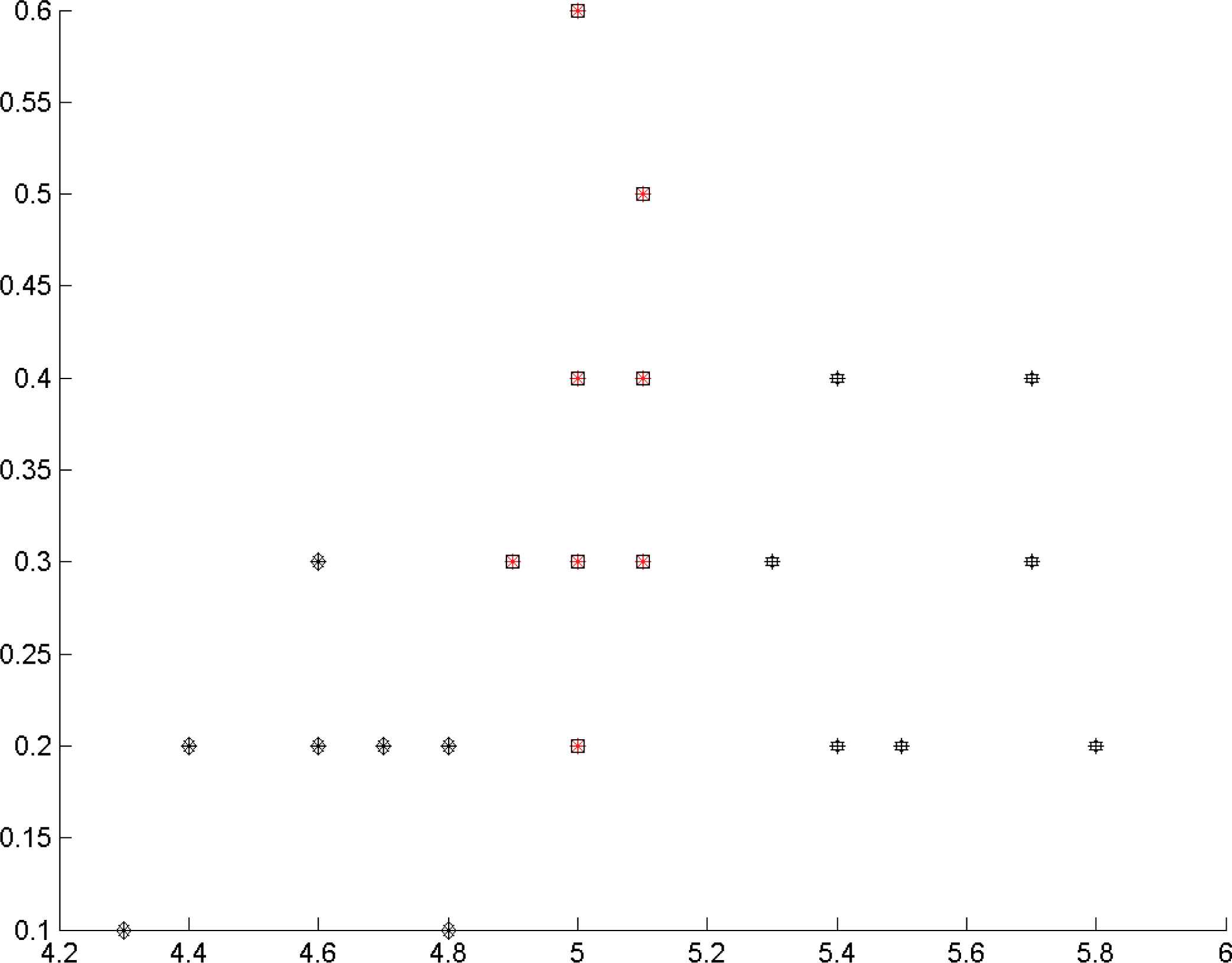
This dataset has been clustered using two clustering algorithms: FCM (with m=1.5) and FCM (with m=2.3), r = 2. Each clustering algorithm has been applied with 9 different parameterizations. We consider 3 kernels (cosine distance, Euclidean distance and Mahalanobis distance) and 3 cluster center initialization methods (random, cumulative approach 26 and subtractive clustering 27).
To demonstrate the process of construction of a H-fuzzy partition, we show in Table 1 the obtained results of the point x = (5,0.3) of cluster 2 from the given data set. We select x = (5,0.3) for illustration because this is a point just between two cluster centers. If we select e.g. x = (4.25,0.1), it is easily clustered into correct cluster. We have two hesitant fuzzy sets H1, H2 and two sets of cluster centers (one for each cluster). In the following steps we construct the H-fuzzy partition:
- •
Cluster alignment. To do so, we compute the correlation coefficient between every pair of hil,hpj for p,i = 1,2 and l, j = 1,2,3 using Eq. (10). Then the derived correlation matrix is:
based on ρ matrix in this example the pairs (h11,h21), (h12,h22) and (h13,h23) are associated. - •
Membership determination for each cluster. Use the average operator in Eq.(7) on the membership values of associated clusters to compute the mean member ship degree for the jth cluster. That is, for each cluster j, j = 1,2,3, compute:
In this example for considering all information we assume that
- •
Definition of H-fuzzy partition. Define a hesitant fuzzy set of clusters for each x ∈ X, H* as follow:
H* is a H-fuzzy partition. Also, we have a set of cluster centers for each cluster as follows:
| x = (5,0.3) | ||
|---|---|---|
| H1(5,0.3):FCM (m = 1.5) | h11 = {0.9641,0.9640,0.0251,0.0250,0.0250,0.0248,0.0131,0.0130,0.0130} |
|
| h12 = {0.9640,0.9637,0.9636,0.0248,0.0248,0.0130,0.0129,0.0129} |
|
|
| h13 = {0.9640,0.9637,0.9636,0.9635,0.0248,0.0248,0.0130,0.0129,0.0129}. |
|
|
| H2(5,0.3):FCM (m = 2.3) | h21 = {0.9614,0.9613,0.9607,0.0256,0.0255,0.0255,0.0135,0.0135,0.0135}, |
|
| h22 = {0.96086,0.96083,0.9607,0.0256,0.0251,0.0251,0.0136,0.0134,0.0134}, |
|
|
| h23 = {0.960863,0.96083,0.96074,0.02565,0.02514,0.01360,0.01342,0.01341}. |
|
|
The clustering values for x = (5,0.3).
In order to evaluate the quality of the final resulting clusters in this H-fuzzy partition, we use the accuracy measure, F score. This measurement evaluates the similarity of a clustering to ground truth information of classes 28. Let m be the number of individual classes. Then, the total F score will be computed as the weighted sum of these classes F score according to their size. The F score can be calculated using Eq. (24), in which Xq is a class with the size of nr and F(Cr) is the F score of the class Xq.
For each class Xq, F(Cr) finds a cluster Si that agrees with Xq better than to the other clusters. F(Cr) is calculated using equation (25), where PSi is the precision (the number of objects in the cluster Si belonging to the class Xq, divided by the number of objects in the cluster Si) and RSi is the recall (the number of objects in the cluster Si belonging to the class Xq, divided by number of objects in the class Xq).
The obtained F score of two executions of FCM (with m = 1.5 and m = 2.3) and H-fuzzy partition on the two dimensional data set and IRIS data set are illustrated in Table (2).
| Dataset | Fscore of |
||
|---|---|---|---|
| H-fuzzy partition | FCM (m=1.5) | FCM (m=2.3) | |
| Iris14 | 1 | 0.8933 | 0.8933 |
| IRIS | 0.9264 | 0.8933 | 0.8933 |
The results of first experiments.
4. Conclusion and Future Works
In this paper, we have introduced a definition for H-fuzzy partitions and proposed a method to define them from fuzzy ones. The definition generalizes I-fuzzy partitions and lets the user apply the reliable membership values and cluster centers for new element in various cluster validity indices. In this paper we consider F score to evaluate the obtained H-fuzzy partition.
References
Cite this article
TY  - JOUR
AU  - Laya Aliahmadipour
AU  - Vicenç Torra
AU  - Esfandiar Eslami
AU  - Mahdi Eftekhari
PY  - 2016
DA  - 2016/06/01
TI  - A Definition for Hesitant fuzzy Partitions
JO  - International Journal of Computational Intelligence Systems
SP  - 497
EP  - 505
VL  - 9
IS  - 3
SN  - 1875-6883
UR  - https://doi.org/10.1080/18756891.2016.1175814
DO  - 10.1080/18756891.2016.1175814
ID  - Aliahmadipour2016
ER  -