
An autonomous teaching-learning based optimization algorithm for single objective global optimization
- DOI
- 10.1080/18756891.2016.1175815How to use a DOI?
- Keywords
- Teaching-Learning Based Optimization; Global Optimization; Autonomy; Learning Desires
- Abstract
Teaching-learning based optimization is a newly developed intelligent optimization algorithm. It imitates the process of teaching and learning simply and has better global searching capability. However, some studies have shown that TLBO is good at exploration but poor at exploitation and often falls into local optimum for certain complex problems. To address these issues, a novel autonomous teaching-learning based optimization algorithm is proposed to solve the global optimization problems on the continuous space. Our proposed algorithm is remodeled according to the three phases of the teaching and learning process, learning from a teacher, mutual learning and self-learning among students instead of two phases of the original one. Moreover, the motivation and autonomy of students are considered in our proposed algorithm, and the expressions of autonomy are formulated. The performance of our proposed algorithm is compared with that of the related algorithms through our experimental results. The results indicate the proposed algorithm performs better in terms of the convergence and optimization capability.
- Copyright
- © 2016. the authors. Co-published by Atlantis Press and Taylor & Francis
- Open Access
- This is an open access article under the CC BY-NC license (http://creativecommons.org/licences/by-nc/4.0/).
1 Introduction
Optimization problems are solved commonly by mathematical methods to obtain the optimal solution, but it is basically very difficult to find the optimal solution within an acceptable time because the optimization problems in practice are NP-hard. Thus, many researchers have proposed some intelligent optimization approaches to optimization problems, and have achieved fruitful results.
Recently, the design principle of intelligent optimization algorithms are generally based on biological behavior, the laws of physics (or phenomena) and human behavior (or cognitive), etc., which are all the innovative design ideas. The algorithms inspired by some biological
TLBO’s design philosophy is relatively new, and it has solved some engineering design problems15,16,17,18, some studies show that TLBO is not among the best meta-heuristics19,20 and has some shortcomings, such as, (i) the design of TLBO is so simple that it only includes two phase, teacher phase and leaner phase. In fact, the process of learning includes learning from teacher, learning from his/her classmates and self-learning. Besides, motivation is a direct factor to affect learning. Some learners maybe have their stronger desires for improving their scores, while others have their weaker motivation. Consequently, the effect of learners depends on their own learning desires, in other words, learning desires can reflect the ability to gain a sense of achievement through learning. This capability of learners is called autonomy in this paper. Obviously, TLBO doesn’t reflect the autonomy of the learners. (ii) TLBO suffers from premature and falls into the local optimum. To avoid the disadvantages of TLBO and to improve the autonomy, we reconstruct an autonomous teaching-learning based optimization, called ATLBO, on the basis of the teaching and learning process.
In our ATLBO, we firstly assume that the teaching-learning process has three phases: learning from teacher, group learning and self-learning. Then, we formulate some expressions according to the characteristics of each learning phase. Finally, we verify the validity of the ATLBO algorithm by means of the extensive experiments.
The main contributions of this paper are presented in the following.
- (i).
We propose a novel behavior-inspired swarm intelligence algorithm on the basis of the teaching and learning process. This population-based optimization algorithm demonstrates an outstanding performance in the global optimization.
- (ii).
We introduce the learning desire into our proposed algorithm to embody the learners’ autonomy.
- (iii).
We carry out a large number of experiments to investigate the effectiveness and efficiency on some classical functions in previous references, and the latest CEC2014 benchmark suite.
The rest of this paper is organized as follows: Section 2 presents the TLBO algorithm proposed by R. V. Rao. Section 3 explains the process how to design the ATLBO algorithm in detail. Section 4 shows simulation results. Finally, conclusions are stated in Section 5.
2 Teaching-learning based Optimization Algorithm
The TLBO algorithm is a population-based optimization algorithm, which was developed according to the teaching and learning. There are two characters in the teaching-learning system, one is a teacher, and the other is learner. The best individual (learner) is viewed as the teacher. Learners learn from the teacher or from another learner. The purpose of the teacher is to improve the average score of a whole class, while the targets of these learners are to increase their own scores. Therefore, TLBO has two phases, i.e., teacher phase and learner phase.
To facilitate the description, we have an example with minimum optimization problem. Let the objective function be f(X) with D -dimensional variables X ∈ [−Rm, +Rm], where −Rm and +Rm are the lower bound and the upper bound of the independent variable X, respectively. Xi = (xi1,xi2,…,xiD) represents the position of the ith learner, i ∈ {1,2,3,…,N}. The teacher is denoted by Xteacher = arg min f(Xj), j ∈ {1,2,3,…,N}. The mean position of all learners
2.1 Teacher phase
During the teacher phase, the teacher imparts knowledge to his/her learners. Then, the position of learner Xi is updated as follows:
If f(X(t)) < f(X(t − 1)), then we accept X(t).
2.2 Learner phase
In the learner phase, learners learn from each other. That is, a learner Xi randomly selects another one Xj(j ≠ i), and interacts with Xj. Then, the learning can be expressed as follows.
2.3 Remove duplicates phase
According to the TLBO description16,17 and the TLBO MATLAB code obtained from its inventors, duplicate elimination step is applied. The duplicate elimination strategy is given in the following.
| Duplicate elimination strategy |
|---|
Foreach duplicate(Pj) do Pj ←random_solution(); Evaluate(Pj); Num_eval + +; If Num_eval + +== MFE then return best(P); End End |
Where duplicate(Pj) indicates that the solution of Pj has existed in the candidate solutions, Num_eval is the number of fitness value evaluation, MFE is the maximum of fitness value evaluations.
Although the TLBO algorithm is a simple and effective method that can solve many optimization problems, it has some unreasonable ideas. TLBO, by nature, is a hill climbing method, and it cannot reflect the autonomy of individual learner. Ref. 21 reported that the performance of TLBO is not better than other EAs. As V. K. Patel pointed out that: “teaching factor of TLBO is relatively fixed, without considering the individual’s self-learning ability” 22. In other words, TLBO doesn’t conform to the teaching and learning in real world. As we all known, the learning, for a learner, should be divided into three types, learning form the teacher, group learning and self-learning. Therefore, we develop an autonomous teaching and learning optimization algorithm provided that the real process of teaching and learning, and the individual learning autonomy are given full consideration, namely ATLBO, which is methodologically different from TLBO.
3 Description of ATLBO
During the actual teaching and learning process, the teacher needs to innovate and to improve their teaching level; learners perform a continuous learning process including learning from the teacher, learning from another learner within his/her group and self-learning so as to raise their own grades. Moreover, as a learner, he/she can take the initiative to learn with a strong or weak learning desire.
As a result, we reconstruct framework of the ATLBO algorithm as follows. There are a number of groups in the class; the learning process of a learner in a group consists of three steps: individual firstly learns from the teacher, then learns from the optimal individual in the group, finally refines himself/herself. In addition, in order to reflect the autonomy of individual, we put forward the concept of learning desire whose magnitude can reflect the intensity property of a learner’s autonomy. Here we also assume that the objective function is f* = min f(X).
3.1 Learning from the teacher
In this phase, learners learn from the teacher (the optimal learner), i.e., learners narrow the distance with their teacher with learning desire. In other words, learners can adjust the search direction and step length in the light of the intensity of their learning desires. Then the learning desire Gi of Xi can be written as
Then Eq (1) can be converted into
3.2 Group learning
During this process, the leaner interact with the optimal learner of his/her group, and narrows the distance from the local optimal individual. Let Xbest be the optimal individual of group K. The interaction of learner Xi and Xbest can be written as
3.3 Self-learning
The goal of self-learning is to increase the ability of the exploitation of the ATLBO algorithm. Because the ergodicity of chaos systems can help to improve the exploitation, we design the self-learning using chaos mapping based on the advantages of chaos. More importantly, we have already started our research in chaos and achieved some results24,25,26,27. All of these studies are based on chaotic ant swarm. Chaotic ant has the chaotic behavior of a single ant and self-organizing ability of the whole ant colony8. Therefore, we devise the self-learning using chaos mapping of an ant. Chaos mapping of an ant8 is Z(t) = Z(t − 1)eμ(1−Z(t−1)). Let
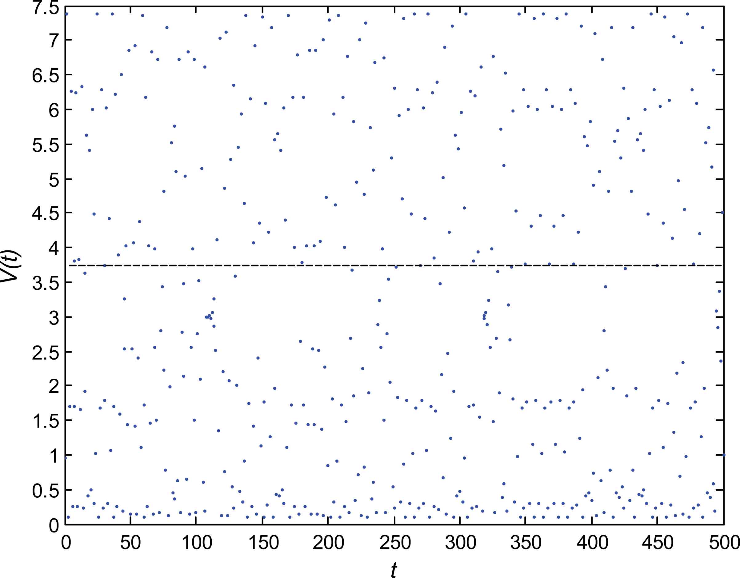
Eq.(8) is chaotic when μ = 3
In order to make the interval [0, 7.5] cover the search interval [−Rm, Rm], we transform Eq. (8) into Eq. (9)
To embody the study motivation, the self-learning desire Si is quantized as follows
3.4 Dynamic study group
To improve the population diversity and to avoid falling into a local optimum, ATLBO uses a strategy of dynamic study group. We discuss three sub-problems in the following: the definition of a dynamic study group, how to reorganize a group and the best time to reorganize the group.
In a class, learners often discuss some problems within a study group which is usually composed of adjacent learners. In order to simulate this kind of learning environment, we construct a two-dimensional grid as shown in Fig 2.
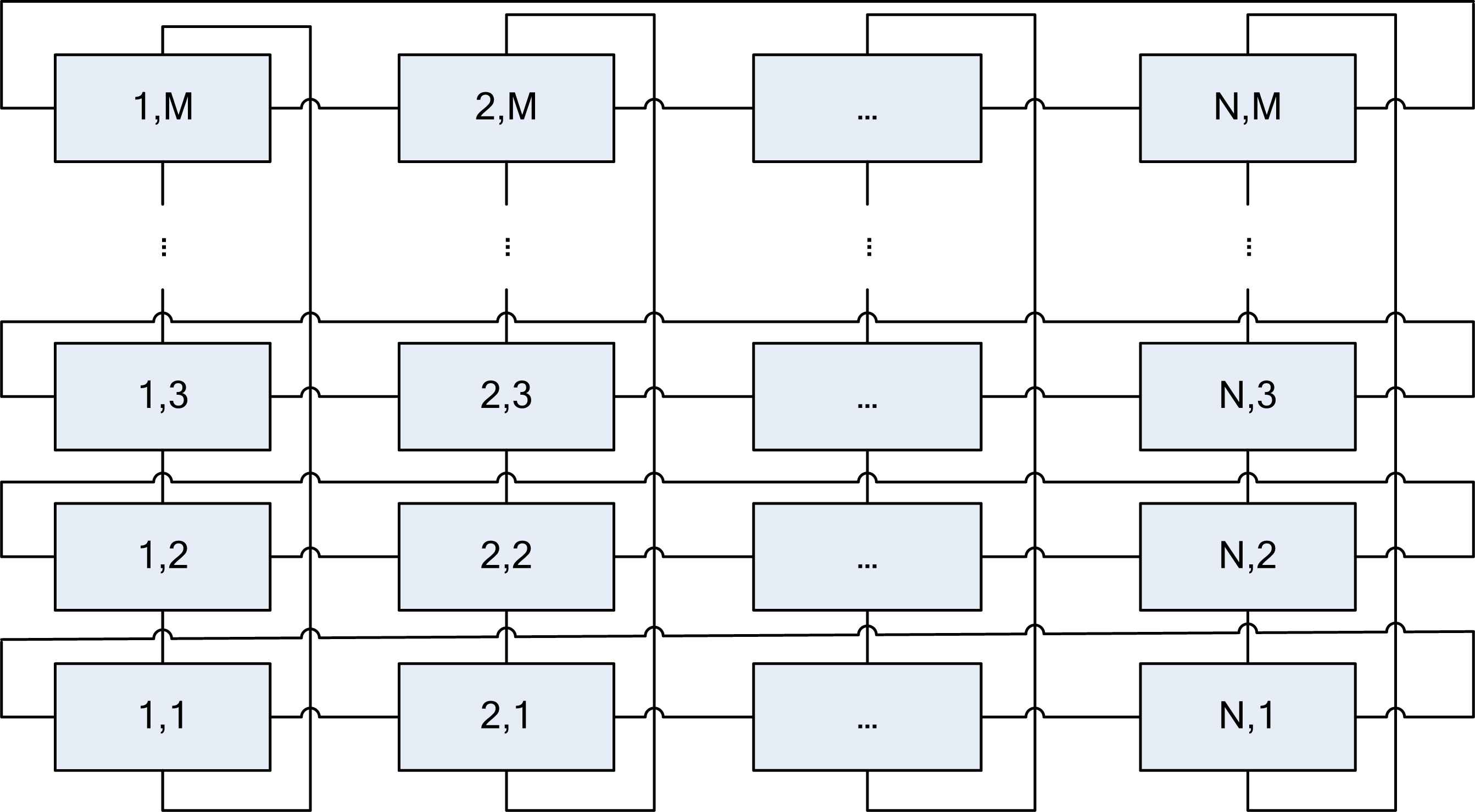
Two-dimensional grid M × N
In the grid, each learner occupies a two-dimensional coordinate. For a learner, its study group is composed of the front, back, left, right learners and itself. Because the study groups mutual overlay each other, the information can be spread to the whole class, and then by means of the interaction among the learners to achieve the purpose of global optimization.
Let Sm,n be the site of learner Xi, then the group of Xi
To improve the diversity of search, we require changing the learner’s position from one study group to another, that is, the position of a learner is changed from one site to another. The 2D mesh is fixed when a learner changes his/her position. For simplicity, we randomly exchange two rows or columns. For example, &(S(r,)),&(S(,l)) are learners of rth row and lth columns. We can exchange two rows &(S(r1,)) and &(S(r2,)) when ALTBO needs, r1, r2 are random integer on the interval [1, M], and |r1 – r2| > 2. Of course, we can exchange two columns &(S(,l1)), &(S(,l2)) by the same token, here l1, l2 are also integer on the interval [1, N], and |l1 − l2| > 2.
During the search process, if the fitness values do not change for two successive times, it may lead to decrease learners’ exploitation ability, especially in the anaphase of the evolutionary process. Therefore, once the aforementioned cases encountered in the evolutionary process, group adjusting strategy is started to improve the search ability.
3.5 Steps of ATLBO
The steps of our ATLBO algorithm can be summarized as follows.
- Step 1:
Initialize the parameters of ATLBO, such as the maximum of fitness value evaluations (MFE), population size(popsize), dimension of variables(n), difficulty factor(α), learning desire Gi(0), self-learning desire Si(0) and so forth. The initial value Xi = {xi,1,xi,2,…,xi,n} is defined as follows:
where xL and xU is the lower and upper boundaries of variables, respectively. - Step 2:
Evaluate each learner f(Xi) and choose the best one to be the teacher with the objective function at current time. Get the learning desire Gi(t) from Eq.(4).
- Step 3:
Calculate TF = round(1 + rand(1)), update all learners according to Eq.(5).
- Step 4:
- Step 5:
Execute the self-learning according to section 3.3, if rand()<Si, accept Xi of self-learning.
- Step 6:
Determine whether the groups are restructured according to subsection 3.4.
- Step 7:
If Num_eval = MFE, terminate ALBO and output the best solution. Otherwise jump Step 2.
Similar to genetic algorithm (GA), ant colony optimization (ACO), artificial bee colony algorithm (ABC)6, ATLBO is a population based optimization. But the most important difference between relevant algorithms and ATLBO in that: (i) ATLBO is constructed based on a learner’s learning process with autonomy; (ii) the learners’ study motivations are taken account in the proposed ATLBO; (iii) reconstructing the study group strategy is applied. Although our ATLBO algorithm is slightly more complicated than TLBO, it is easy to implement, moreover, it employs a novel design idea.
Besides the common parameters such as population size popsize, dimension of variables n etc., there are three control parameters of ATLBO: the difficulty factor α, learning desire Gi and self-learning desire Si. According to Eq. (4), we can see from that a lager α may guide ATLBO to explore a larger area, while a small α may make ATLBO execute a more intensive exploitation. As for Gi and Si, they can improve the best solutions and can increase the autonomy of each learner. Empirically, we recommend setting α to 1.03, Gi(0) to 0.62, Si(0) to 1.
4 Simulation experiments
To verify the performance of our ATLBO algorithm, we devise two types of experiments, one is for the global convergence of the proposed algorithm, and the other is for the effectiveness of our algorithm. For fairness, we compare ATLBO with several classic algorithm, such as artificial bee colony algorithm (ABC)6, CLPSO 28, TLBO14, ETLBO17. All algorithms run on a computer of Intel Core i5 2.50GHz CPU, 4GB memory, Matlab 7.14. In a two-dimensional grid of learning environment, the number of columns is 6, and the number of rows is 10. The maximum and minimum weights of CLPSO are 0.9 and 0.4 respectively, and the number of ETLBO’s elite individual is set to 4. The code of ABC is from http://mf.erciyes.edu.tr/abc, and that of ETLBO is from https://sites.google.com/site/tlborao. In additions, our stop criterion is the number of fitness value evaluations instead of the number of iterations, and the relevant parameters of other algorithms are in accordance with the corresponding papers.
4.1 Comparison of Convergence Speed
Convergence tests are firstly done as follows. For fair comparison, we use 18 benchmark functions which are come from Ref.29,30,31,32. The 18 benchmark functions are listed in table 1. In table 1, f1 − f5 are multimodal functions, f6 − f10 are unimodal functions, the remained functions f11 − f18 are rotated models. The “Range” in table 1 is the interval of the variables, “fmin” is the optimal solution, “Acceptance” indicates the acceptable solutions of different functions.
| Function | Formula | Range | fmin | Acceptance |
|---|---|---|---|---|
| f1(Weierstrass) |
|
[0.5,0.5] | 0 | 1E-5 |
| f2(Rastigin) |
|
[-5.12,5.12] | 0 | 50 |
| f3 (Rosenbrock) |
|
[-30,30] | 0 | 50 |
| f4(Griewank) |
|
[-600,600] | 0 | 1E-5 |
| f5(Ackley) |
|
[-32.768,32.768] | 0 | 1E-5 |
| f6 (Sum Square) |
|
[-100,100] | 0 | 1E-5 |
| f7(Quadric) |
|
[-100,100] | 0 | 1E-5 |
| f8(Zakharov) |
|
[-10,10] | 0 | 1E-5 |
| f9 (Schwefel’s p2.22) |
|
[-10,10] | 0 | 1E-5 |
| f10(Sphere) |
|
[-100,100] | 0 | 1E-2 |
| f11 (Rotated Quadric) |
|
[-100,100] | 0 | 1E-5 |
| f12 (Rotated Zakharov) |
|
[-10,10] | 0 | 1E-5 |
| f13 (Rotated Schwefel’s p2.22) |
|
[-10,10] | 0 | 1E-5 |
| f14 (Rotated Rosenbrock) |
|
[-2.048,2.048] | 0 | 50 |
| f15 (Rotated Ackley) |
|
[-32.768,32.768] | 0 | 1E-5 |
| f16 (Rotated Rastrigin) |
|
[-5.12,5.12] | 0 | 50 |
| f17 (Rotated Weierstrass) |
|
[0.5,0.5] | 0 | 1E-5 |
| f18 (Rotated Griewank) |
|
[-600,600] | 0 | 1E-5 |
The 18 benchmark functions
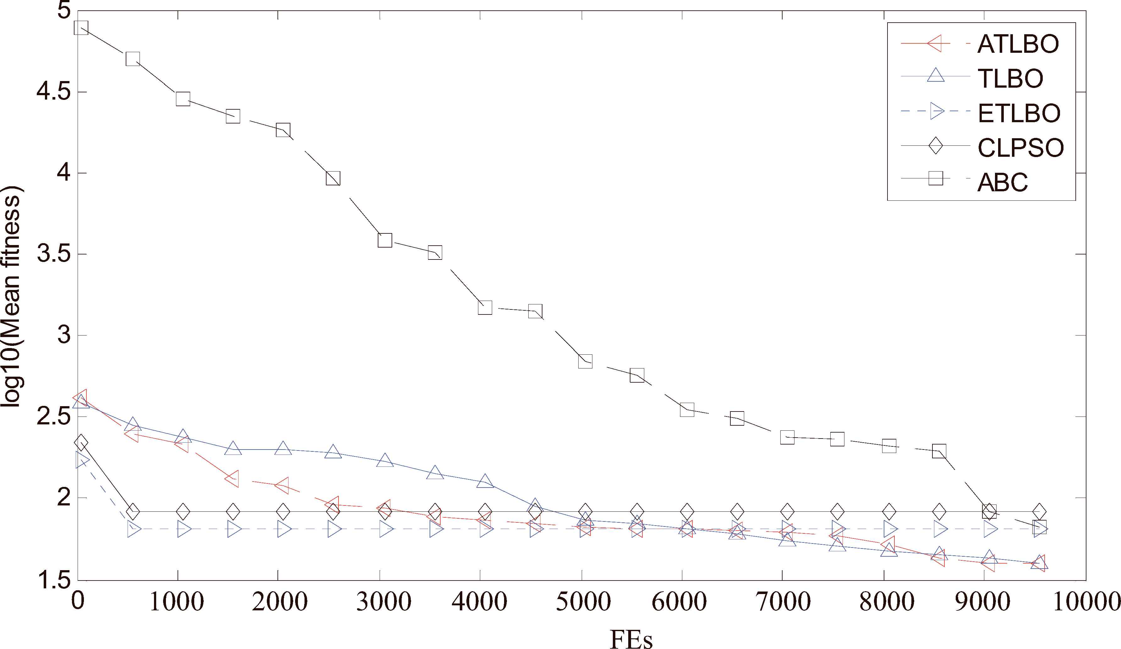
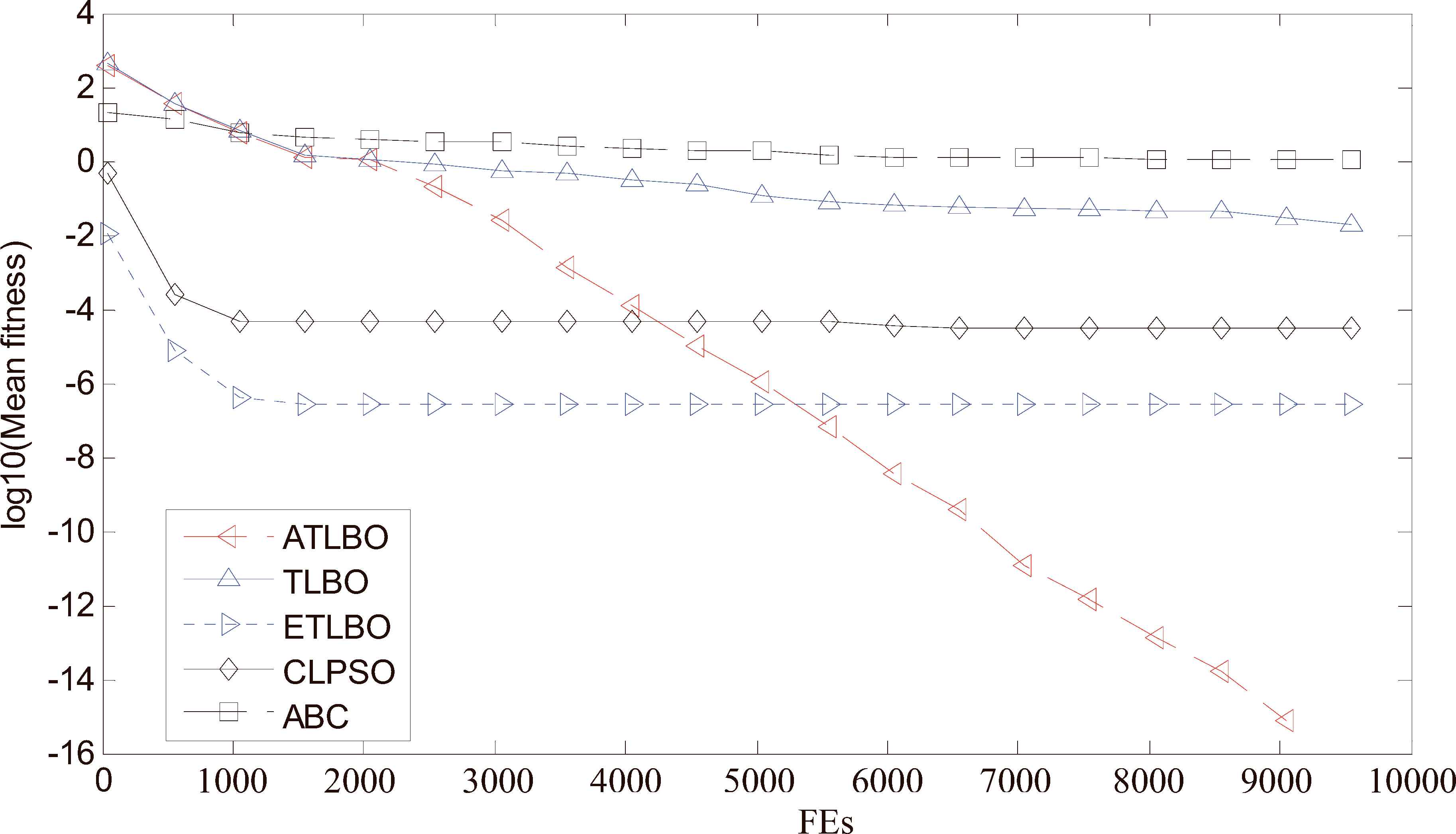
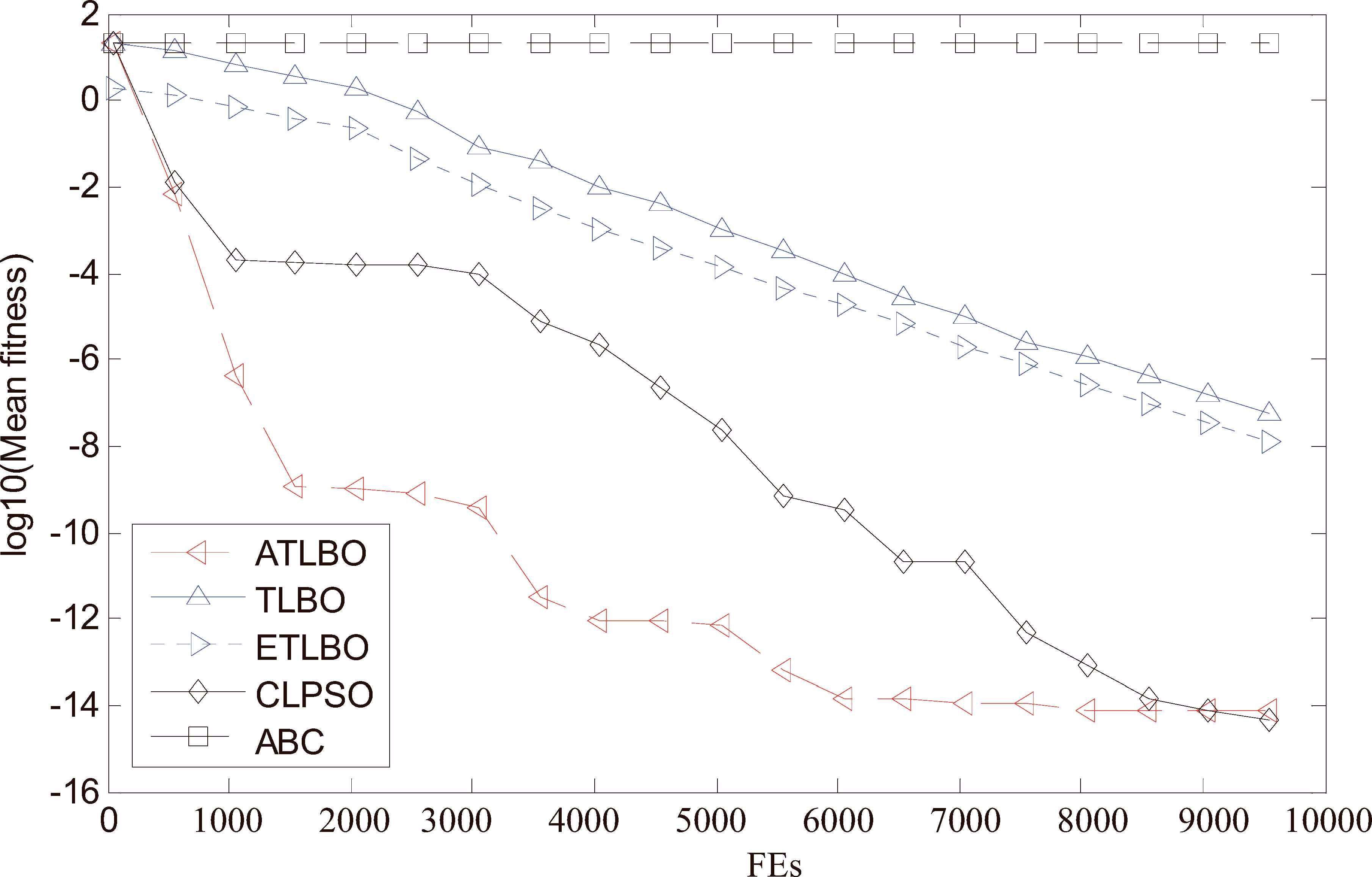
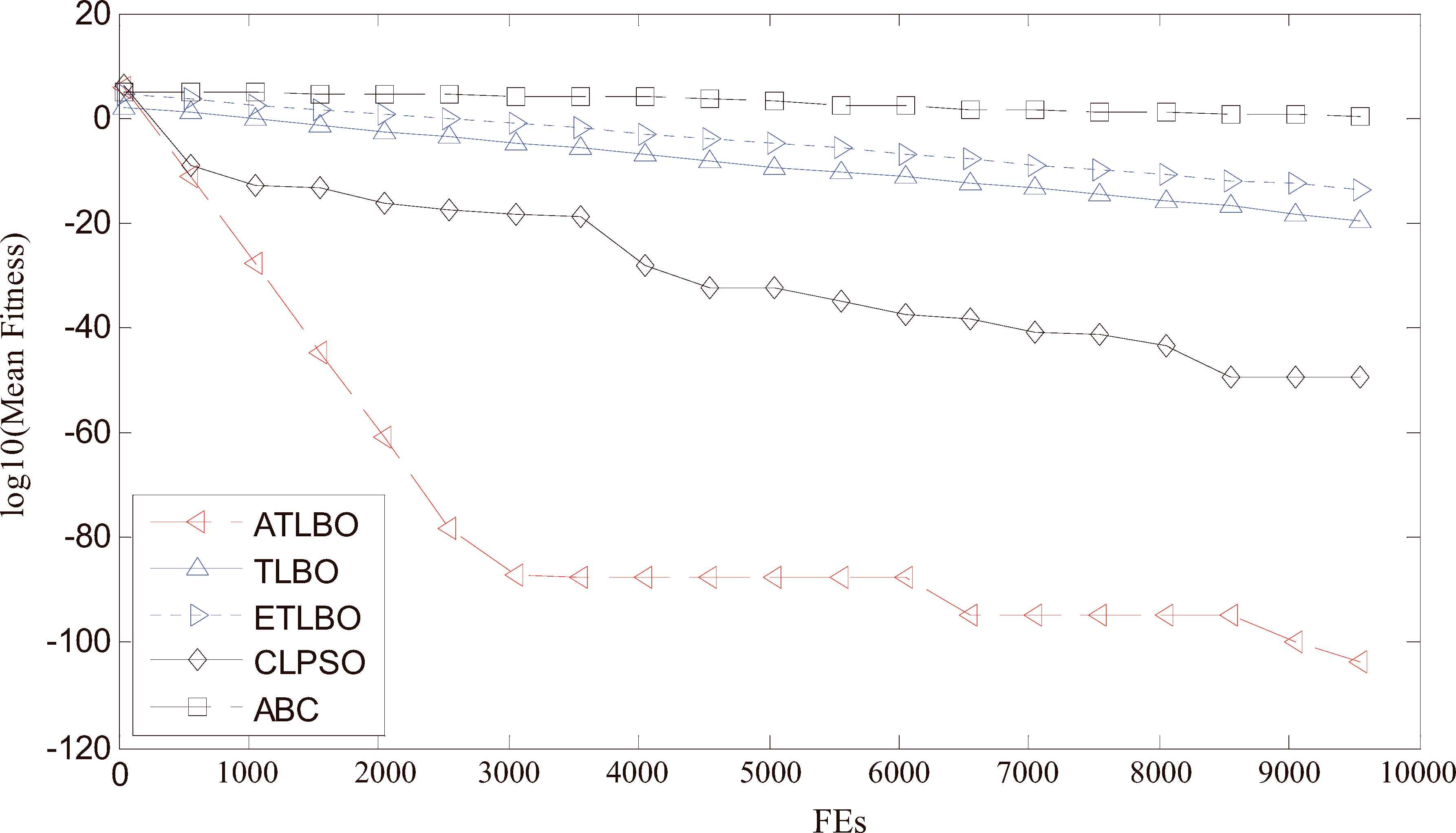
All algorithms are run 50 independently on 18 functions with 30-dimension in accordance with related literatures. We also take a measure of these functions’ convergence in Table 1 by the mean fitness values. Due to space limitations, here are the optimization processes of five algorithms on 5 functions f2, f3, f4, f5, f10 with 30 dimensions as shown in Figures 3–7. In Figures 3–7, the vertical axis is the average fitness value of 50 times, and the horizontal axis is the number of fitness value evaluations (FEs), and MFE = 10000.
Convergence performance of the 5 different algorithms on 30 dimensional f2 (Rastigin) function.
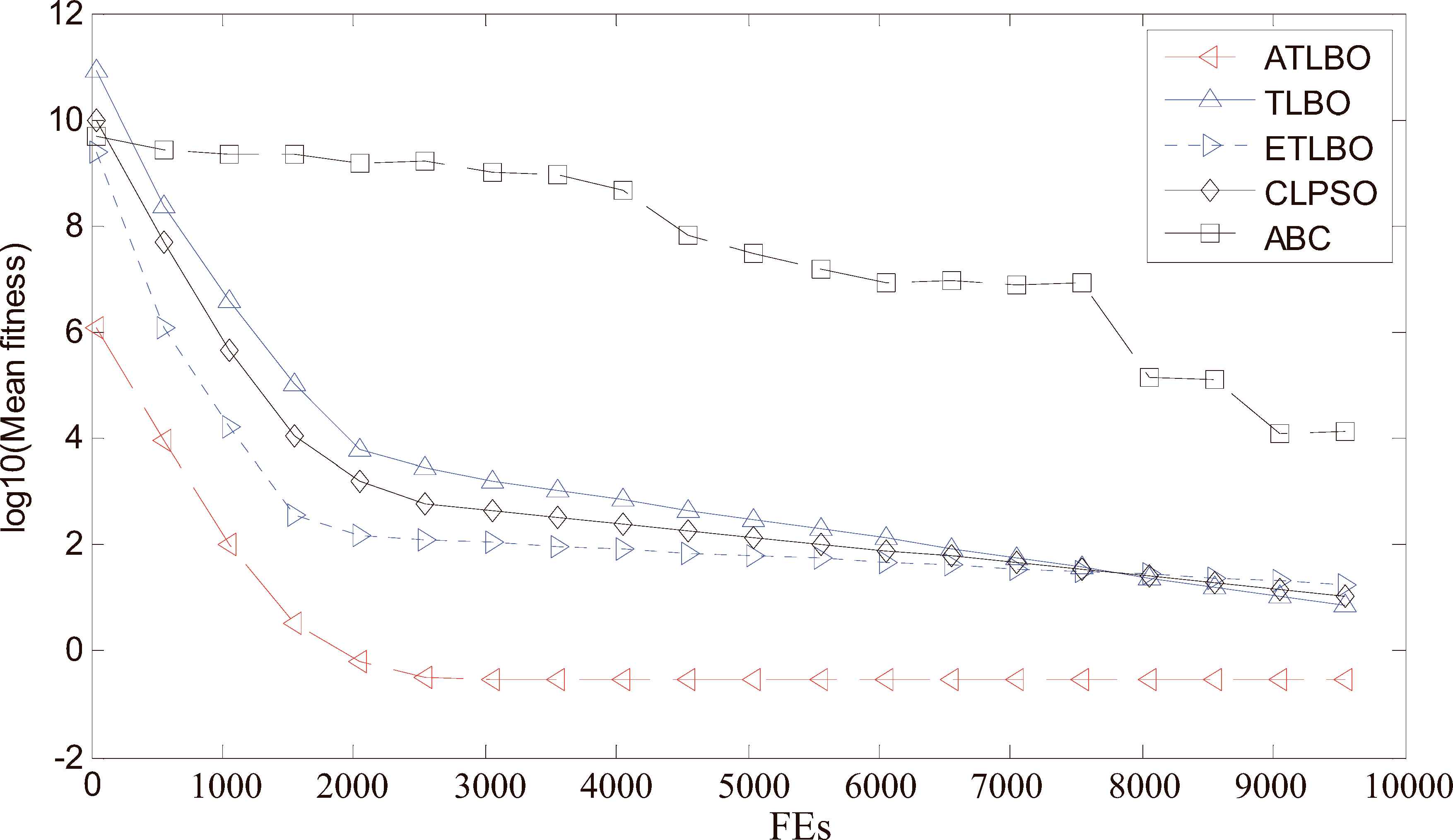
Convergence performance of the 5 different algorithms on 30 dimensional f3 (Rosenbrock) function.
Convergence performance of the 5 different algorithms on 30 dimensional f4 (Griewank) function.
Convergence performance of the 5 different algorithms on 30 dimensional f5 (Ackley) function.
Convergence performance of the 5 different algorithms on 30 dimensional f10 (Sphere) function.
It can be seen from Figs. 3 to 7 that: (i) the proposed ATLBO algorithm shows a greater advantage over other four algorithms especially for Sphere, Griewank, Rosenbrock and Schwefel functions; (ii) ATLBO has faster convergence, showing strong optimization ability for Sphere, Rosenbrock, Ackley and Schwefel functions. These results show ATLBO are effective for the unimodal and multimodal functions.
4.2 comparison of solution accuracy
As we all known, the solution accuracy is a salient yardstick for an algorithm. Therefore, we carry out the accuracy tests by two sets of benchmark functions, the first set is the 18 functions in table 1, and the other set is 30 benchmark functions of the CEC 2014 competition on single objective real-parameter numerical optimization33. The CEC’14 benchmark suite is summarized in Table 2, which includes various types of function optimization problems. Although the second set (CEC’14) is more complete and contains harder problems—shifted and rotated functions than the first set functions, here we still give comparative results of the first set in order to facilitate to compare with the previous papers for readers. All these 30 functions’ search range are [-100,100]D. In order to distinguish the functions from the table 1, each function in table 2 will be recognized by the capital letter “F”. More complete descriptions are in Ref. 33.
| Type | ID | Function | Fi = Fi(X*) |
|---|---|---|---|
| Unimodal | F1 | Rotated High Conditioned Elliptic Function | 100 |
| F2 | Rotated Bent Cigar Function | 200 | |
| F3 | Rotated Discus Function | 300 | |
| Multimodal | F4 | Shifted and Rotated Rosenbrock’s Function | 400 |
| F5 | Shifted and Rotated Ackley’s Function | 500 | |
| F6 | Shifted and Rotated Weierstrass Function | 600 | |
| F7 | Shifted and Rotated Griewank’s Function | 700 | |
| F8 | Shifted Rastrigin’s Function | 800 | |
| F9 | Shifted and Rotated Rastrigin’s Function | 900 | |
| F10 | Shifted Schwefel’s Function | 1000 | |
| F11 | Shifted and Rotated Schwefel’s Function | 1100 | |
| F12 | Shifted and Rotated Katsuura Function | 1200 | |
| F13 | Shifted and Rotated HappyCat Function | 1300 | |
| F14 | Shifted and Rotated HGBat Function | 1400 | |
| F15 | Shifted and Rotated Expanded Griewank’s plusRosenbrock’s Function | 1500 | |
| F16 | Shifted and Rotated Expanded Scaffer’s F6 Function | 1600 | |
| Hybrid | F17 | Hybrid Function 1 (N=3) | 1700 |
| F18 | Hybrid Function 2 (N=3) | 1800 | |
| F19 | Hybrid Function 3 (N=4) | 1900 | |
| F20 | Hybrid Function 4 (N=4) | 2000 | |
| F21 | Hybrid Function 5 (N=5) | 2100 | |
| F22 | Hybrid Function 6 (N=5) | 2200 | |
| Composition | F23 | Composition Function 1 (N=5) | 2300 |
| F24 | Composition Function 2 (N=3) | 2400 | |
| F25 | Composition Function 3 (N=3) | 2500 | |
| F26 | Composition Function 4 (N=5) | 2600 | |
| F27 | Composition Function 5 (N=5) | 2700 | |
| F28 | Composition Function 6 (N=5) | 2800 | |
| F29 | Composition Function 7 (N=3) | 2900 | |
| F30 | Composition Function 8 (N=3) | 3000 |
The 30 CEC’14 test functions
4.2.1 Solution accuracy tests using the 18 benchmark functions
In these tests, we set the maximum number of fitness evaluations (FEs) to 20000 for every algorithm to ensure a sufficient comparison. Every algorithm has been run 50 times on every test function with 30 dimensions to reduce the occurrence of statistical errors. The best, mean solution and standard deviation of the 50 trails are listed in Table 3. The best solutions of these algorithms are indicated with boldface.
| Function | ABC | CLPSO | TLBO | ETLBO | ATLBO | |
|---|---|---|---|---|---|---|
| f1 | Best | 0.00E+00 | 8.65E-03 | 0.00E+00 | 0.00E+00 | 0.00E+00 |
| Mean | 9.18E-15 | 1.17E-02 | 0.00E+00 | 0.00E+00 | 0.00E+00 | |
| Std. | 6.67E-15 | 9.74E-04 | 0.00E+00 | 0.00E+00 | 0.00E+00 | |
| f2 | Best | 578E-15 | 1.79E-01 | 6.85E+00 | 0.00E+00 | 0.00E+00 |
| Mean | 4.08E-12 | 3.14E-01 | 1.42E+01 | 2.34E+01 | 1.17E+01 | |
| Std. | 1.25E-11 | 9.47E-02 | 5.23E+00 | 1.27E+01 | 9.81E+00 | |
| f3 | Best | 7.98E+00 | 2.37E+01 | 1.85E+01 | 2.12E+01 | 2.95E+00 |
| Mean | 1.43E+01 | 2.74E+01 | 1.96E+01 | 2.21E+01 | 7.02E+00 | |
| Std. | 3.78E+00 | 4.51E+00 | 7.58E-01 | 6.45E-01 | 2.04E+00 | |
| f4 | Best | 0.00E+00 | 1.98E-04 | 0.00E+00 | 0.00E+00 | 0.00E+00 |
| Mean | 5.78E-16 | 4.22E-04 | 0.00E+00 | 0.00E+00 | 0.00E+00 | |
| Std. | 7.98E-16 | 2.01E-04 | 0.00E+00 | 0.00E+00 | 0.00E+00 | |
| f5 | Best | 6.37E-13 | 2.55E-03 | 3.23E-15 | 3.18E-15 | 2.13E-16 |
| Mean | 1.42E-12 | 3.50E-03 | 3.45E-15 | 3.53E-15 | 2.05E-16 | |
| Std. | 3.82E-13 | 8.12E-04 | 0.00E+00 | 0.00E+00 | 0.00E+00 | |
| f6 | Best | 4.45E-16 | 9.38E-05 | 0.00E+00 | 0.00E+00 | 0.00E+00 |
| Mean | 6.17E-16 | 1.78E-04 | 0.00E+00 | 0.00E+00 | 0.00E+00 | |
| Std. | 1.13E-16 | 7.19E-05 | 0.00E+00 | 0.00E+00 | 0.00E+00 | |
| f7 | Best | 5.98E+03 | 4.73E+03 | 5.42E-84 | 7.21E-146 | 0.00E+00 |
| Mean | 8.07E+03 | 7.12E+03 | 4.76E-81 | 7.56E-144 | 0.00E+00 | |
| Std. | 9.12E+02 | 1.59E+03 | 2.19E-80 | 2.18E-143 | 0.00E+00 | |
| f8 | Best | 3.92E+02 | 4.87E+01 | 1.58E-52 | 4.78E-147 | 0.00E+00 |
| Mean | 3.76E+02 | 8.45E+01 | 2.45E-51 | 5.61E-144 | 0.00E+00 | |
| Std. | 6.94E+01 | 1.47E+01 | 3.49E-51 | 1.78E-142 | 0.00E+00 | |
| f9 | Best | 2.14E-14 | 3.12E-04 | 1.35E-184 | 2.14E-176 | 0.00E+00 |
| Mean | 3.75E-14 | 4.09E-04 | 3.94E-181 | 3.45E-175 | 0.00E+00 | |
| Std. | 7.45E-15 | 1.63E-05 | 1.85E-181 | 2.78E-175 | 0.00E+00 | |
| f10 | Best | 2.83E-16 | 5.74E-06 | 0.00E+00 | 0.00E+00 | 0.00E+00 |
| Mean | 4.78E-16 | 1.81E-05 | 0.00E+00 | 0.00E+00 | 0.00E+00 | |
| Std. | 1.24E-16 | 5.88E-06 | 0.00E+00 | 0.00E+00 | 0.00E+00 | |
| f11 | Best | 5.23E+03 | 4.37E+03 | 1.75E-86 | 2.34E-151 | 0.00E+00 |
| Mean | 7.46E+03 | 7.35E+03 | 1.45E-80 | 2.34E-140 | 0.00E+00 | |
| Std. | 1.68E+03 | 1.78E+03 | 6.42E-80 | 5.34E-140 | 0.00E+00 | |
| f12 | Best | 3.45E+02 | 7.55E+01 | 2.01E-57 | 5.82E-127 | 0.00E+00 |
| Mean | 4.75E+02 | 9.40E+01 | 5.36E-52 | 1.93E-123 | 0.00E+00 | |
| Std. | 7.06E+01 | 2.19E+01 | 1.23E-51 | 2.13E-123 | 0.00E+00 | |
| f13 | Best | 1.23E-03 | 1.42E-01 | 4.19E-181 | 2.84E-175 | 0.00E+00 |
| Mean | 1.39E-02 | 2.27E-01 | 1.45E-178 | 3.94E-173 | 0.00E+00 | |
| Std. | 1.32E-02 | 7.67E-02 | 7.21E-179 | 5.12E-173 | 0.00E+00 | |
| f14 | Best | 1.30E+01 | 2.19E+01 | 1.56E+01 | 1.24E+01 | 2.34E+00 |
| Mean | 2.77E+01 | 2.01E+01 | 3.54E+01 | 4.53E+01 | 2.81E+00 | |
| Std. | 1.72E+01 | 7.21E-01 | 2.16E+01 | 2.13E+01 | 3.01E+00 | |
| f15 | Best | 6.32E-03 | 6.82E-02 | 7.44E-15 | 3.55E-15 | 3.55E-15 |
| Mean | 3.86E-01 | 2.05E-01 | 5.29E-01 | 3.55E-15 | 3.55E-15 | |
| Std. | 5.21E-01 | 7.34E-02 | 6.91E-01 | 0.00E+00 | 0.00E+00 | |
| f16 | Best | 4.12E+01 | 3.76E+01 | 4.87E+00 | 0.00E+00 | 0.00E+00 |
| Mean | 5.81E+01 | 6.12E+01 | 2.13E+01 | 4.38E+01 | 2.61E+01 | |
| Std. | 1.21E+01 | 1.36E+01 | 6.32E+00 | 1.64E+01 | 3.19E-01 | |
| f17 | Best | 5.18E+00 | 6.35E+00 | 0.00E+00 | 0.00E+00 | 0.00E+00 |
| Mean | 5.69E+00 | 7.56E+00 | 0.00E+00 | 0.00E+00 | 0.00E+00 | |
| Std. | 2.34E+00 | 1.67E+00 | 0.00E+00 | 0.00E+00 | 0.00E+00 | |
| f18 | Best | 5.43E-09 | 1.25E-03 | 0.00E+00 | 0.00E+00 | 0.00E+00 |
| Mean | 4.52E-06 | 3.45E-03 | 0.00E+00 | 0.00E+00 | 0.00E+00 | |
| Std. | 6.54E-06 | 5.64E-03 | 0.00E+00 | 0.00E+00 | 0.00E+00 |
The best, mean solutions and standard deviation of the 50 trials obtained by various methods on 30 dimensional functions.
Table 3 shows that ATLBO has advantage over the other approaches in terms of the best, mean solution and standard deviation on the unimodal functions f6, f7, f8, f9, f10. Except for functions f2, f3, the proposed ATLBO algorithm has obtained some better solution. For function f2, the best solution of ATLBO are smaller than those of other methods, while the mean solution and standard deviation of ATLBO can’t match those of other methods. As for function f3, ATLBO outperforms the other algorithms in terms of the best and mean solution, but it is inferior to the other algorithms in terms of standard deviation. For rotated test functions f11 − f18, ATLBO also has a significant advantage except for functions f14, f16. For functions f11 − f14, the performance of ATLBO has better than that of TLBO and ETLBO.
Table 3 demonstrates the ATLBO has best performance, and the second is ETLBO. The optimal solutions of ATLBO are the same as the theoretical optimums for functions f1, f2, f4, f6, f7, f8, f9, f10, f11, f12, f13, f17, f18, For functions f3, f14, f15, f16, ATLBO is worse than others, but it has closely performance with the other algorithms. These experimental results prove right the theorem of ‘no free lunch’34, one algorithm cannot outperform all the others on every aspect.
For a though comparison, the t-test is adopted for statistical analysis. Table 4 presents the T values and the P values on every function of this two-tailed test with a significant level of 0.05 between ATLBO and another algorithm. The boldface shows that the performance of ATLBO is better than those of other algorithm in terms of T values and P values. The “Better”, “Same” and “Worse” indicate the number of functions that ATLBO performs significantly better than, almost the same as, and significantly worse than the compared algorithm, respectively. “Merits” represents the difference between the number of “Better” and the number of “Worse”.
| Function | ABC | CLPSO | TLBO | ETLBO | |
|---|---|---|---|---|---|
| f1 | T | 7.4117 | 64. 6883 | 0. 0000 | 0. 0000 |
| p | 0.0000 | 0. 0000 | 0. 0000 | 0. 0000 | |
| f2 | T | -6.4227 | −6. 2500 | 1. 2110 | 3. 9262 |
| p | 0.0000 | 0. 0000 | 0. 2308 | 0. 0002 | |
| f3 | T | 9.1271 | 22. 1720 | 31. 1291 | 37. 9560 |
| p | 0.0000 | 0. 0000 | 0. 0000 | 0. 0000 | |
| f4 | T | 3.9005 | 11. 3062 | 0. 0000 | 0. 0000 |
| p | 0.0003 | 0. 0000 | 0. 0000 | 0. 0000 | |
| f5 | T | 20.0153 | 23. 2119 | 0. 0000 | 0. 0000 |
| p | 0.0000 | 0. 0000 | 0. 0000 | 0. 0000 | |
| f6 | T | 29.4040 | 13. 3318 | 0. 0000 | 0. 0000 |
| p | 0.0000 | 0. 0000 | 0. 0000 | 0. 0000 | |
| f7 | T | 47.6516 | 24. 1147 | 1. 1705 | 1. 8675 |
| p | 0.0000 | 0. 0000 | 0. 2466 | 0. 0669 | |
| f8 | T | 29.1761 | 30. 9555 | 3. 7804 | 0. 1697 |
| p | 0.0000 | 0. 0000 | 0. 0004 | 0. 8658 | |
| f9 | T | 27.1065 | 135. 1247 | 0. 0000 | 0. 0000 |
| p | 0.0000 | 0. 0000 | 0. 0000 | 0. 0000 | |
| f10 | T | 20.7589 | 16. 5768 | 0. 0000 | 0. 0000 |
| p | 0.0000 | 0. 0000 | 0. 0000 | 0. 0000 | |
| f11 | T | 23.9127 | 22. 2365 | 1. 2163 | 2. 3598 |
| p | 0.0000 | 0. 0000 | 0. 2288 | 0. 0217 | |
| f12 | T | 36.2316 | 23. 1144 | 2. 3467 | 4. 8795 |
| p | 0.0000 | 0. 0000 | 0. 0224 | 0. 0000 | |
| f13 | T | 5.6707 | 15. 9378 | 0. 0000 | 0. 0000 |
| p | 0.0000 | 0. 0000 | 0. 0000 | 0. 0000 | |
| f14 | T | 7.6762 | 30. 0824 | 8. 0474 | 10. 6368 |
| p | 0.0000 | 0. 0000 | 0. 0000 | 0. 0000 | |
| f15 | T | 3.9898 | 15. 0403 | 4. 1227 | 0. 0000 |
| p | 0.0002 | 0. 0000 | 0. 0001 | 0. 0000 | |
| f16 | T | 14.2368 | 13. 8947 | -4. 0848 | 5. 8109 |
| p | 0.0000 | 0. 0000 | 0. 0001 | 0. 0000 | |
| f17 | T | 13.0947 | 24. 3784 | 0. 0000 | 0. 0000 |
| p | 0.0000 | 0. 0000 | 0. 0000 | 0. 0000 | |
| f18 | T | 3.7219 | 3. 2941 | 0. 0000 | 0. 0000 |
| p | 0.0004 | 0. 0017 | 0. 0000 | 0. 0000 | |
| Best | 18 | 18 | 5 | 6 | |
| Same | 0 | 0 | 12 | 12 | |
| Worst | 0 | 0 | 1 | 0 | |
| Merits | 18 | 18 | 4 | 6 | |
Comparisons of ATLBO and other algorithms on t-test on 30 dimensional functions.
Table 4 displays that the numbers of “Merits” of ABC and CLPSO are all 18, those of TLBO and ETLBO are 4 and 6, respectively. Moreover, the performance of ATLBO is the same as TLBO and ETLBO on 12 functions. Overall, ATLBO almost can obtain the optimum on 18 functions.
4.2.2 Solution accuracy tests using the 30 CEC’14 benchmark functions
In these tests, we use the CEC’14 test suite because “they have several features such as novel basic problems, composing test problems by extracting features dimension-wise from several problems, graded level of linkages, rotated trap problems, and so on” 33. To ensure a fair comparison, we set the maximum number of fitness evaluations (FEs) to 150,000 for each algorithm. Each algorithm has been executed 51 runs on each test functions, as in Ref. 33. Our evaluation of every problem is the average of 51 runs.
The comparative results on unimodal, multimodal, hybrid and composition fucntions are presented respectively in Table 5–8. “max” and “min” respectively refer to the maximum and minimum fitness values of 5 algorithms on every function among the 51 runs. “median” means the median among those of experimental fitness values. “std” denotes the standard deviation of an algorithm on a function. The best results of these comparative algorithms on each function are shown in bold. We also list the statistic test results between ATLBO and other algorithms using two-sided Wilcoxon rank-sum test to check the significance of the difference in Table 9. The h values for every function are presented in Table 9. When h=1, it means that there is a significant difference between the algorithm at the significance level 0.05, and h=-1 vice versa; when h=0, it implies there is no difference.
| Function | ABC | CLPSO | TLBO | ETLBO | ATLBO | |
|---|---|---|---|---|---|---|
| F1 | max | 2.56E+06 | 7.98E+07 | 5.42E+07 | 1.36E+07 | 1.21E+06 |
| min | 3.78E+06 | 5.77E+06 | 4.57E+06 | 1.59E+06 | 1.35E+06 | |
| median | 1.43E+06 | 2.15E+07 | 8.36E+06 | 5.09E+06 | 6.31E+05 | |
| std | 5.47E+05 | 1.68E+07 | 1.33E+07 | 2.72E+06 | 2.51E+05 | |
| F2 | max | 3.94E+04 | 8.05E+06 | 1.59E+04 | 3.12E+04 | 1.51E+03 |
| min | 5.98E+03 | 1.15E+06 | 3.51E+03 | 3.10E+02 | 2.01E+02 | |
| median | 1.53E+04 | 3.84E+06 | 8.41E+03 | 9.10E+03 | 2.78E+02 | |
| std | 6.61E+03 | 1.61E+06 | 3.91E+03 | 6.10E+03 | 2.12E+02 | |
| F3 | max | 1.49E+04 | 4.97E+04 | 7.84E+04 | 3.45E+03 | 1.27E+03 |
| min | 3.49E+03 | 5.87E+02 | 1.96E+04 | 2.99E+02 | 3.08E+02 | |
| median | 7.31E+03 | 6.95E+03 | 4.50E+04 | 3.13E+02 | 4.53E+02 | |
| std | 2.72E+03 | 1.35E+04 | 1.12E+04 | 5.42E+02 | 1.85E+02 |
Comparative results on unimodal benchmark functions.
| Function | ABC | CLPSO | TLBO | ETLBO | ATLBO | |
|---|---|---|---|---|---|---|
| F4 | max | 5.38E+02 | 6.49E+02 | 8.52E+02 | 5.59E+04 | 5.39E+02 |
| min | 4.03E+02 | 4.21E+02 | 5.69E+02 | 2.16E+03 | 3.99E+02 | |
| median | 4.99E+02 | 5.43E+02 | 6.97E+02 | 3.11E+03 | 4.01E+02 | |
| std | 3.81E+01 | 3.45E+02 | 5.23E+01 | 1.81E+03 | 3.71E+01 | |
| F5 | max | 5.24E+02 | 5.20E+02 | 5.20E+02 | 5.21E+02 | 5.20E+02 |
| min | 5.22E+02 | 5.20E+02 | 5.23E+02 | 5.21E+02 | 5.20E+02 | |
| median | 5.22E+02 | 5.20E+02 | 5.23E+02 | 5.21E+02 | 5.20E+02 | |
| std | 4.01E-03 | 4.23E-03 | 6.51E-03 | 7.71E-03 | 6.97E-04 | |
| F6 | max | 6.13E+02 | 6.23E+02 | 6.35E+02 | 6.29E+02 | 5.95E+02 |
| min | 6.02E+02 | 6.10E+02 | 6.31E+02 | 6.21E+02 | 5.85E+02 | |
| median | 6.06E+02 | 6.14E+02 | 6.27E+02 | 6.23E+02 | 5.90E+02 | |
| std | 2.58E+00 | 4.31E+00 | 1.85E+00 | 1.82E+00 | 1.12E+00 | |
| F7 | max | 7.01E+02 | 7.01E+02 | 7.02E+02 | 7.00E+02 | 7.00E+02 |
| min | 7.01E+02 | 7.01E+02 | 7.02E+02 | 7.00E+02 | 7.00E+02 | |
| median | 7.01E+02 | 7.01E+02 | 7.02E+02 | 7.00E+02 | 7.00E+02 | |
| std | 1.23E-02 | 2.59E-02 | 9.63E-02 | 5.64E-02 | 1.20E-03 | |
| F8 | max | 8.69E+02 | 9.42E+02 | 8.17E+02 | 9.65E+02 | 8.23E+02 |
| min | 8.28E+02 | 8.92E+02 | 8.05E+02 | 9.12E+02 | 8.02E+02 | |
| median | 8.45E+02 | 9.24E+02 | 8.12E+02 | 9.38E+02 | 8.15E+02 | |
| std | 5.10E+01 | 3.10E+01 | 2.05E+01 | 1.32E+01 | 2.15E+00 | |
| F9 | max | 9.76E+02 | 9.78E+02 | 1.23E+03 | 1.21E+03 | 9.25E+02 |
| min | 9.32E+02 | 9.64E+02 | 1.03E+03 | 8.79E+02 | 9.01E+02 | |
| median | 9.51E+02 | 9.72E+02 | 1.14E+03 | 1.01E+03 | 9.12E+02 | |
| std | 1.24E+01 | 1.35E+01 | 1.75E+01 | 2.57E+01 | 1.15E+01 | |
| F10 | max | 3.58E+03 | 1.02E+03 | 5.34E+03 | 3.19E+03 | 2.69E+03 |
| min | 1.48E+03 | 1.02E+03 | 3.51E+03 | 1.29E+03 | 1.12E+03 | |
| median | 2.67E+03 | 1.02E+03 | 4.64E+03 | 2.71E+03 | 1.47E+03 | |
| std | 3.82E+02 | 6.80E+01 | 3.71E+02 | 4.23E+02 | 3.58E+02 | |
| F11 | max | 3.81E+03 | 4.49E+03 | 6.45E+03 | 4.32E+03 | 3.91E+03 |
| min | 1.47E+03 | 2.13E+03 | 3.81E+03 | 2.37E+03 | 2.72E+03 | |
| median | 2.98E+03 | 3.12E+03 | 4.57E+03 | 8.56E+03 | 3.43E+03 | |
| std | 4.51E+02 | 5.09E+02 | 5.72E+02 | 5.18E+02 | 2.87E+02 | |
| F12 | max | 1.20E+03 | 1.20E+03 | 1.20E+03 | 1.20E+03 | 1.20E+03 |
| min | 1.21E+03 | 1.20E+03 | 1.21E+03 | 1.20E+03 | 1.20E+03 | |
| median | 1.21E+03 | 1.20E+03 | 1.21E+03 | 1.20E+03 | 1.20E+03 | |
| std | 1.51E-02 | 5.48E-02 | 6.57E-02 | 5.51E-02 | 1.13E-02 | |
| F13 | max | 1.30E+03 | 1.30E+03 | 1.30E+03 | 1.30E+03 | 1.30E+03 |
| min | 1.30E+03 | 1.30E+03 | 1.30E+03 | 1.30E+03 | 1.30E+03 | |
| median | 1.30E+03 | 1.30E+03 | 1.30E+03 | 1.30E+03 | 1.30E+03 | |
| std | 6.49E-02 | 5.59E-02 | 4.41E-02 | 3.42E-02 | 1.89E-02 | |
| F14 | max | 1.42E+03 | 1.40E+03 | 1.40E+03 | 1.40E+03 | 1.40E+03 |
| min | 1.42E+03 | 1.40E+03 | 1.42E+03 | 1.41E+03 | 1.40E+03 | |
| median | 1.42E+03 | 1.40E+03 | 1.42E+03 | 1.41E+03 | 1.40E+03 | |
| std | 1.21E-02 | 1.96E-02 | 4.23E-02 | 1.38E-02 | 1.21E-01 | |
| F15 | max | 1.51E+03 | 1.55E+03 | 1.51E+03 | 1.53E+03 | 1.50E+03 |
| min | 1.51E+03 | 1.51E+03 | 1.51E+03 | 1.51E+03 | 1.50E+03 | |
| median | 1.51E+03 | 1.51E+03 | 1.51E+03 | 1.52E+03 | 1.50E+03 | |
| std | 8.48E-01 | 4.86E+00 | 5.30E+00 | 3.26E+00 | 6.68E-01 | |
| F16 | max | 1.62E+03 | 1.63E+03 | 1.61E+03 | 1.61E+03 | 1.61E+03 |
| min | 1.62E+03 | 1.61E+03 | 1.61E+03 | 1.61E+03 | 1.61E+03 | |
| median | 1.62E+03 | 1.61E+03 | 1.61E+03 | 1.61E+03 | 1.61E+03 | |
| std | 6.17E-01 | 5.72E-01 | 3.45E-01 | 5.41E-01 | 2.23E-01 |
Comparative results on multimodal benchmark functions.
| Function | ABC | CLPSO | TLBO | ETLBO | ATLBO | |
|---|---|---|---|---|---|---|
| F17 | max | 3.48E+05 | 2.29E+07 | 1.21E+06 | 1.12E+06 | 6.12E+04 |
| min | 5.41E+03 | 1.31E+06 | 1.83E+05 | 1.43E+04 | 6.72E+03 | |
| median | 6.65E+04 | 3.12E+06 | 5.61E+05 | 1.52E+03 | 2.72E+04 | |
| std | 6.83E+04 | 4.20E+06 | 2.25E+05 | 1.71E-01 | 1.24E+02 | |
| F18 | max | 1.79E+04 | 1.01E+05 | 4.21E+03 | 1.11E+06 | 2.71E+03 |
| min | 2.31E+03 | 6.81E+03 | 2.03E+03 | 1.45E+04 | 1.78E+03 | |
| median | 4.42E+03 | 2.31E+03 | 2.14E+03 | 1.54E+05 | 2.02E+03 | |
| std | 3.70E+03 | 1.81E+04 | 3.80E+02 | 1.59E+05 | 1.25E+02 | |
| F19 | max | 1.92E+03 | 1.97E+03 | 2.01E+03 | 2.02E+03 | 1.92E+03 |
| min | 1.89E+03 | 1.92E+03 | 1.92E+03 | 1.92E+03 | 1.90E+03 | |
| median | 1.95E+03 | 1.94E+03 | 2.01E+03 | 1.97E+03 | 1.91E+03 | |
| std | 3.70E+00 | 2.79E+01 | 3.45E+01 | 3.32E+01 | 1.42E+00 | |
| F20 | max | 5.41E+03 | 8.64E+04 | 6.83E+04 | 5.98E+04 | 1.57E+04 |
| min | 2.31E+03 | 8.65E+03 | 2.34E+03 | 2.13E+04 | 2.15E+03 | |
| median | 3.45E+03 | 2.73E+04 | 1.78E+04 | 3.65E+04 | 4.35E+03 | |
| std | 7.02E+02 | 1.79E+04 | 1.42E+04 | 8.51E+03 | 3.19E+03 | |
| F21 | max | 8.97E+04 | 1.68E+06 | 3.12E+05 | 1.67E+05 | 1.78E+05 |
| min | 6.81E+03 | 6.71E+04 | 5.67E+04 | 1.02E+04 | 3.72E+03 | |
| median | 3.36E+04 | 4.23E+05 | 1.82E+05 | 4.72E+04 | 2.93E+04 | |
| std | 2.31E+04 | 3.36E+05 | 6.63E+04 | 4.31E+04 | 3.51E+04 | |
| F22 | max | 2.56E+03 | 3.30E+03 | 3.71E+03 | 3.77E+03 | 2.86E+03 |
| min | 2.24E+03 | 2.26E+03 | 2.71E+03 | 2.41E+03 | 2.23E+03 | |
| median | 2.37E+03 | 2.72E+03 | 3.17E+03 | 3.10E+03 | 2.51E+03 | |
| std | 7.41E+01 | 2.41E+02 | 2.48E+02 | 2.68E+02 | 1.45E+02 |
Comparative results on hybrid benchmark functions.
| Function | ABC | CLPSO | TLBO | ETLBO | ATLBO | |
|---|---|---|---|---|---|---|
| F23 | max | 2.63E+03 | 2.58E+03 | 2.66E+03 | 2.62E+03 | 2.62E+03 |
| min | 2.58E+03 | 2.58E+03 | 2.51E+03 | 2.62E+03 | 2.62E+03 | |
| median | 2.61E+03 | 2.58E+03 | 2.59E+03 | 2.62E+03 | 2.62E+03 | |
| std | 9.85E-02 | 1.22E+00 | 6.39E+01 | 2.63E+03 | 1.61E-01 | |
| F24 | max | 2.64E+03 | 2.66E +03 | 2.72E+03 | 2.62E+03 | 2.60E+03 |
| min | 2.61E+03 | 2.63E+03 | 2.63E+03 | 2.63E+03 | 2.60E+03 | |
| median | 2.62E +03 | 2.65E+03 | 2.67E+03 | 6.92E+00 | 2.60E+03 | |
| std | 1.09E +01 | 5.98E+03 | 1.26E+01 | 2.63E+03 | 1.67E-02 | |
| F25 | max | 2.69E+03 | 2.71E+03 | 2.72E+03 | 2.75E+03 | 2.74E+03 |
| min | 2.68E+03 | 2.71E+03 | 2.71E+03 | 2.71E+03 | 2.71E+03 | |
| median | 2.69E+03 | 2.71E+03 | 2.71E+03 | 2.73E+03 | 2.73E+03 | |
| std | 9.31E-01 | 3.01E+03 | 1.34E+00 | 6.31E+00 | 2.13E+00 | |
| F26 | max | 2.86E+03 | 2.80E+03 | 2.79E+03 | 2.76E+03 | 2.70E+03 |
| min | 2.70E+03 | 2.70E+03 | 2.79E+03 | 2.72E+03 | 2.70E+03 | |
| median | 2.81E+03 | 2.70E+03 | 2.79E+03 | 2.74E+03 | 2.70E+03 | |
| std | 5.62E+01 | 2.23E+01 | 6.43E-02 | 3.45E+00 | 5.12E-02 | |
| F27 | max | 3.62E+03 | 3.54E+03 | 4.23E+03 | 6.51E+03 | 3.50E+03 |
| min | 3.12E+03 | 3.25E+03 | 3.15E+03 | 3.45E+03 | 3.10E+03 | |
| median | 3.45E+03 | 3.41E+03 | 3.91E+03 | 4.95E+03 | 3.10E+03 | |
| std | 3.42E+01 | 7.80E+01 | 3.61E+02 | 6.75E+02 | 4.85E+01 | |
| F28 | max | 3.79E+03 | 5.67E+03 | 6.92E+03 | 6.62E+03 | 5.41E+03 |
| min | 3.61E+03 | 3.62E+03 | 4.62E+03 | 4.69E+03 | 3.59E+03 | |
| median | 3.70E+03 | 5.58E+03 | 5.12E+03 | 5.61E+03 | 4.70E+03 | |
| std | 4.09E+01 | 8.56E+01 | 5.61E+02 | 4.59E+01 | 3.78E+02 | |
| F29 | max | 2.81E+04 | 8.94E+06 | 4.23E+07 | 2.86E+06 | 5.28E+03 |
| min | 5.47E+03 | 5.34E+03 | 5.75E+03 | 3.12E+03 | 3.45E+03 | |
| median | 1.60E+04 | 6.34E+03 | 3.41E+04 | 3.14E+03 | 4.12E+03 | |
| std | 5.26E+03 | 1.34E+05 | 7.86E+06 | 3.75E+05 | 3.74E+02 | |
| F30 | max | 1.73E+04 | 3.75E+04 | 1.23E+05 | 3.75E+04 | 7.68E+03 |
| min | 7.52E+03 | 7.12E+03 | 1.32E+04 | 8.37E+03 | 4.32E+03 | |
| median | 8.92E+03 | 1.59E+03 | 1.52E+04 | 1.52E+04 | 5.61E+03 | |
| std | 2.30E+03 | 6.09E+03 | 1.85E+04 | 6.75E+03 | 7.41E+02 |
Comparative results on composition benchmark functions.
| F1 | F2 | F3 | F4 | F5 | F6 | F7 | F8 | F9 | F10 | F11 | F12 | F13 | F14 | F15 | |
| ABC(h) | 1 | 1 | 1 | 1 | 1 | −1 | 1 | 1 | −1 | 1 | −1 | 0 | 0 | 0 | 1 |
| CLPSO(h) | 1 | 1 | 1 | 1 | 1 | 1 | 1 | 1 | −1 | −1 | 0 | 0 | 1 | 1 | 1 |
| TLBO(h) | 1 | 1 | 1 | 1 | −1 | 1 | 0 | 0 | 1 | 1 | 1 | 0 | 1 | 1 | 0 |
| ETLBO(h) | 1 | 1 | −1 | 1 | 1 | 1 | 1 | 1 | 1 | 1 | 0 | 0 | 1 | 1 | 1 |
| F16 | F17 | F18 | F19 | F20 | F21 | F22 | F23 | F24 | F25 | F26 | F27 | F28 | F29 | F30 | |
| ABC(h) | 0 | 1 | 1 | 0 | −1 | 0 | −1 | 1 | −1 | −1 | 1 | 0 | −1 | 1 | 1 |
| CLPSO(h) | −1 | 1 | 1 | 1 | 1 | 1 | 1 | 1 | 1 | 1 | 1 | 1 | 0 | 1 | 1 |
| TLBO(h) 1 | 1 | 1 | 1 | 1 | 1 | 1 | 0 | −1 | −1 | 1 | 1 | 1 | −1 | 1 | |
| ETLBO(h) | 1 | 1 | 1 | 1 | 1 | 1 | 1 | 1 | 1 | 1 | 1 | 1 | 1 | 1 | 1 |
Comparisons between ATLBO and other algorithms using two-sided Wilcoxon rank-sum test with significance level 0.05.
The comparative results on unimodal benchmark functions are given in Table 5. Table 5 shows that ATLBO obtains the best median values and the smallest standard deviation on F1 and F2, and those on F3 are next to ETLBO, while ATLBO obtains the smallest standard deviation on F3. According to the statistic tests in Table 9, the experimental results of the proposed ATLBO are significantly different from the other four methods on F1 and F2, and different from the other three methods except for ETLBO on F3. It is obvious that ATLBO outperforms better than the other algorithms in spite of these rotated trap problems.
Table 6 presents the comparative results on multimodal functions F14 − F16. In Table 6, ATLBO can get the best median values on 9 functions. CLPSO ranks second, and obtains the best median values on six functions, while ETLBO ranks third, obtains the best median values on three functions, TLBO only obtains the best values on one function. Especially, both CLPSO and ATLBO achieve the maximum performance on functions F5, F12, F14, F16. Seen from Table 9, ATLBO has significant differences from or equal to the other algorithms on functions F1, F2, F4, F7, F8, F13, F14, F15, F17, F18, F19, F21, F23, F26, F27, F30. While ATLBO has no statistically significant different from CLPSO on functions F9, F10.
Comparisons of hybrid functions are presented in Table 7. From Table 7, ATLBO obtains the best median values on five functions F17, F18, F19, F21, F22, and obtains the second best median value on F20, which is slightly less than that of ABC. Note that these functions are hybrid by different basic functions, which maybe cause some algorithms reducing their performance significantly such as CLPSO, TLBO and ETLBO, on the contrary, ATLBO still keeps its competition.
Table 8 presents the comparative results on composition functions F23 − F30. ATLBO obtains the best median values on F24, F26, F27, F30. CLPSO obtains the best median value on F23, but it loses the first place in terms of the standard deviation, ABC ranks first on F25. When we cast our eyes at Table 9, we can see that the relatively low performance of ATLBO on F25, F28, which sets from that the composition group functions have a large number of local optima.
From Table 4–9, we can draw a conclusion that ATLBO offers significant performance over the other five algorithms on CEC2014 benchmark suite, but sometimes ATLBO loses its advantages on a few test functions with too many local optima.
Through the above analysis, the obtained results reveal that ATLBO exhibits the best performance on whole experiments but not always. In fact, no algorithm can be better than all other algorithms, i.e., every algorithm has its strength and weakness. Of course, we apply some suitable strategies so that our algorithm can avoid some defects35.
Compared with those algorithms highly ranked in the CEC2014 competition, ATLBO performs better. That is because that most of competitive algorithms have apply complicated mechanisms, such as mutation operator, control parameter 36, hybrid strategies, hyper-heuristic controllers, parameter fine-turning mechanism, etc.. However, our objection is to test the basic performance of ATLBO on the benchmark suite. The next researches improve the performance of ATLBO by introducing appropriate strategies or integrating with effective operator from other algorithms.
5 Conclusions
In this paper, we proposed an autonomous teaching-learning based optimization (ATLBO) to solve single objective global optimization. This algorithm is reconstructed according to the teaching and learning process, learning from teacher, group learning and self-learning. Combined with the teaching-learning based optimization, group learning and self-learning methods are introduced. Group learning increases the exploration of TLBO, and self-learning improves the exploitation of TLBO. In order to evaluate the performance of ATLBO, we adopt two sets of benchmark functions which cover a larger variety of different optimization problem types. We compared ATLBO with the state-of-the-art optimization algorithm, namely, ABC, CLPSO, TLBO and ETLBO. As shown in the simulation results, the solution search quality of the ATLBO is generally better than that of other algorithms.
Future research on ATLBO can be divided into two categories: algorithm research and real-world application. For the first, we will focus on designing more efficient search strategy to improve the exploration and exploitation of ATLBO, and give exploitation and exploration measure; for the second, we address some real-word applications using ATLBO effectively and efficiently.
Acknowledgements
The authors would like to thank the editor and all the anonymous reviewers for their valuable comments and suggestions that improved the paper’s quality. This work is partially supported by Natural Science Foundation of Anhui Province, China (Grant No. 1408085MF130), and the Education Department of Anhui Province Natural Science Foundation (Grant Nos. KJ2013A229, KJ2013Z281). The authors would like to thank Prof. Suganthan, Prof. Karaboga and Prof. Rao for providing some algorithms codes.
References
Cite this article
TY  - JOUR
AU  - Fangzhen Ge
AU  - Liurong Hong
AU  - Li Shi
PY  - 2016
DA  - 2016/06/01
TI  - An autonomous teaching-learning based optimization algorithm for single objective global optimization
JO  - International Journal of Computational Intelligence Systems
SP  - 506
EP  - 524
VL  - 9
IS  - 3
SN  - 1875-6883
UR  - https://doi.org/10.1080/18756891.2016.1175815
DO  - 10.1080/18756891.2016.1175815
ID  - Ge2016
ER  -