
Adopting Relational Reinforcement Learning in Covering Algorithms for Numeric and Noisy Environments
- DOI
- 10.1080/18756891.2016.1175819How to use a DOI?
- Keywords
- Covering Algorithm; RULES Family; Continuous Features; Relational Reinforcement Learning
- Abstract
Covering algorithms (CAs) constitute a type of inductive learning for the discovery of simple rules to predict future activities. Although this approach produces powerful models for datasets with discrete features, its applicability to problems involving noisy or numeric (continuous) features has been neglected. In real-life problems, numeric values are unavoidable, and noise is frequently produced as a result of human error or equipment limitations. Such noise affects the accuracy of prediction models and leads to poor decisions. Therefore, this paper studies the problem of CAs for data with numeric features and introduces a novel non-discretization algorithm called RULES-CONT. The proposed algorithm uses relational reinforcement learning (RRL) to resolve the current difficulties when addressing numeric and noisy data. The technical details of the algorithm are thoroughly explained to demonstrate that RULES-CONT contribute upon the RULES family by collecting its own knowledge and intelligently re-uses previous experience. The algorithm overcomes the infinite-space problem posed by numeric features and treats these features similarly to those with discrete values, while incrementally discovering the optimal rules for dynamic environments. It is the first RRL algorithm that intelligently induces rules to address continuous and noisy data without the need for discretization or pruning. To support our claims, RULES-CONT is compared with 7 well-known algorithms applied to 27 datasets with four levels of noise using 10-fold cross-validation, and the results are analyzed using box plots and the Friedman test. The results show that the use of RRL results in significantly improved noise resistance compared with all other algorithms and reduces the computation time of the algorithm compared with the preceding version, which does not use relational representation.
- Copyright
- © 2016. the authors. Co-published by Atlantis Press and Taylor & Francis
- Open Access
- This is an open access article under the CC BY-NC license (http://creativecommons.org/licences/by-nc/4.0/).
1. Introduction
Currently, intelligent machines can be found in almost every home around the world. Data are collected by these machines, and decisions are made depending on user behavior. Machine learning (ML) is one of the tools that can be used for this purpose1, and a significant amount of research has focused on the concept of classification learning. Although statistical methods are widely used in ML, various studies2, 3 have shown that these methods are very difficult to understand and act as black boxes. Another subset of ML techniques, called covering algorithms (CAs)4, possess several characteristics that make them more attractive than statistical ML methods. The basic purpose of a CA is to learn a set of rules from a given set of instances and create a classifier that can predict new situations. This approach is interesting because of its simplicity and direct representations, which are unambiguous and can be easily updated, understood and validated.5–7 Unfortunately, CAs face one major hurdle that makes it difficult to apply them to real-life problems.
CAs are essentially designed to address discrete and clean values, whereas problems involving noise or quantities that can take any values in an infinite space have been neglected. However, the ability to handle numeric (continuous)1 features is important for addressing complex real-life problems. In the literature regarding CAs, several attempts have been made to solve this problem, but suitable solutions are still lacking. ElGibreen and Aksoy8 investigated the problem in various inductive learning (IL) families. According to the summary of the state of the art presented in that paper, numeric features were originally handled by means of discretization; the deficiencies of these approaches can be summarized as follows:
- •
Offline Discretization: Future updates are a major concern because it is difficult to update the intervals of older rules; this difficulty reduces their accuracy.
- •
Online Discretization: More accurate than offline discretization, but its time and computational costs are very high because a large number of evaluations must be performed during the learning stage.
Within the past few years, another approach has been developed by a small group of researchers. It is called non-discretization because it does not involve the discretization of features and addresses both numeric and discrete values in the same manner. Although this approach overcomes some of the problems with discretization, it also encounters new issues, as follows:
- •
Non-discretization: This approach overfit its training sets, resulting in a reduced level of noise tolerance. Current methods attempt to address this problem using pruning techniques, but this increases the complexity of the algorithm, and it is difficult to determine the appropriate pruning technique to use.
To address the issues discussed above, this paper focuses on the problem of noise tolerance in a dataset with numeric features. The primary goal is to generalize the performance of CAs for application to numeric datasets such that good results can be obtained even if noise is introduced. This objective was chosen because it is important to build a repository that can address real-world problems, especially considering that noise is typically present in the data collected to address such problems. Whether these data are collected from users or gathered through sensors, noise is frequently produced as a result of limitations in the measurement equipment or through human error. Such noise affects the accuracy of prediction models, which can cause agents to make poor decisions.
This paper contributes to the field of CAs by introducing the use of relational reinforcement learning (RRL) in a CA family called RULES9. A novel non-discretization approach using RRL is proposed, and based on this approach an algorithm called RULES with continuous attributes (RULES-CONT) is developed. This algorithm scales to any type of data, fills the gaps in CA applications, and discovers simple and strong knowledge that can be used by both expert systems and decision-makers.
Unlike other versions of RULES, the proposed algorithm uses the concept of knowledge transfer 10, 11in order to incrementally update its repository. It re-uses past rules discovered in previous steps to incrementally update the repository when a new patch of data is provided as input. Transferred knowledge that covers any of the new examples is stored in the new repository, and the covered example is flagged for no further processing. This increases the speed of the algorithm and takes advantage of historical experience. The induction procedure is different from that of all other algorithms in the family; although it induces one rule at a time, induced rule is discovered using RRL procedure. In RULES-CONT, the RRL process is adjusted to discover the optimal rules using a reward function. The features and their possible values are stored in logical representations, and the agent continuously learns the best optimal rule values via trial-and-error interactions.
To the best of our knowledge, no one has previously exploited RRL to solve the problem of applying CAs to data with numeric features. The RRL elements are adapted to the problem of rule induction in CAs and to discover the best actions to induce the optimal rule for every seed example. Through the use of RRL, the algorithm is endowed with several appealing properties in addition to the ability to solve problems with numeric features. Because RRL has the property of continuous learning, the extracted knowledge can be easily updated without the need for additional procedures. Thus, it becomes possible to automatically update the repository if incremental induction is applied.
To test the performance of RULES-CONT, the KEEL tool12, 13 was used for 10-fold cross-validation. The proposed algorithm was compared with seven different algorithms applied to 27 real-life benchmarks. The error rates of the algorithms at four levels of noise were collected to assess the noise resistance in the case of datasets with numeric features. Moreover, the total resistance level was visualized using box plots, and the total variance in the error rate over all levels of noise was computed. Afterward, the Friedman test was applied to determine whether there were significant differences in performance and to rank the algorithms using the CD diagram. Finally, to demonstrate how the use of RRL representation reduces the computation time of the algorithm, the speed of RULES-CONT was compared with that of the preceding non-discretization version, in which RRL is not applied. The results confirm that the RRL approach offers significantly improved noise resistance and that the use of the relational representation reduces the computation time.
This paper is organized as follows: First, the fundamentals of CAs and RRL elements are defined followed by a discussion of related work on the problem of numeric datasets. Then, the proposed algorithm is discussed, along with its technical details. Next, the performance of the algorithm is benchmarked, and the empirical results are discussed. Finally, the paper concludes with perspectives on future work.
2. Preliminaries
This section defines the CA problem and presents the elements required to build RRL agent.
2.1. Covering Algorithms
CAs are often called separate-and-conquer algorithms because they separate each instance or example when inducing optimal rules. The resulting rules are stored in an ‘IF condition THEN conclusion’ structure. One example (called a seed) is selected at a time to incrementally build a rule, condition by condition.
Problem Statement -
The problem of rule induction in a CA can be mathematically expressed as in (1), where the CA is described in terms of four characteristics: E, A, V and CF. E represents the finite set of examples (instances) provided as input to the agent. A is the finite set of features (attributes) possessed by each example. Note that the last feature is the class and represents the output to be predicted in the future. V denotes the infinite set of values that can be taken by each feature in each example, which represents a feature domain. This domain may consist of either discrete or numeric values. Finally, CF is the classifier that represents the conclusions drawn based on the presented data, which are stored as rules in the CA.
For example, Table 1 shows a dataset that can be given to a classifier for the construction of a model. The contents of this table represent the problem of user satisfaction with a purchased laptop, in which the purpose is to predict whether users will be satisfied with their laptops. The table contains three seed examples and five features. In this example, E comprises each row; A includes Disk Space, Battery Life, Price, RAM and Satisfied, where Satisfied is the class; the values (V) of the features are shown in each cell and include both discrete (nominal) and continuous (numeric) values; and CF is the set of rules induced from this table.
| Disk Space | Battery | Price | RAM | Satisfied |
|---|---|---|---|---|
| 3 | High | 5000 | 5i | No |
| 4 | High | 6000 | 7i | Yes |
| 6 | Medium | 3000 | 7i | Yes |
CA data sample for user satisfaction on laptops
2.2. Relational Reinforcement Learning (RRL)
Reinforcement learning (RL) is inspired by the manner in which a living being learns to behave through interacting with its environment. Kaelbling et al.14 state that RL is “the problem faced by an agent that must learn behavior through trial-and-error interactions with a dynamic environment”. The main goal of RL is to reach a decision through a series of tasks involving trial-and-error interactions with the environment.15 In RL, learners are not told what to do but instead discover the most rewarding actions by trying them.
Based on the concept of RL, an extension of RL called RRL was developed for better space representation16. It was developed to facilitate the handling of a large number of states and actions by grouping them into one object. In RRL tasks, relational atoms are used to describe the environment16–18. One of the best-known representations for this purpose is relational factoring, which uses abstract qualities in first-order logic (FOL). Mellor19 conducted several studies and concluded that the primary advantage of this approach is its simplicity due to static abstraction.
Definition –
Given the following elements, the objective RRL is to find a policy π that selects actions rA from the state space rS and maximizes the total rewards16. Thus, any state is actually an r-state that consists of multiple states connected by a logical operation, and the action space is also an r-action space that contains relevant actions within the state space.20
- 1.
A set of states S ∈ rS is described in relational language and belongs to the state rS.
- 2.
A set of actions A ∈ rA is described in relational language, and each state has its own set of actions.
- 3.
A real-valued reward (r: S × A → R) to determine whether the agent has chosen a good action.
Example – Blocks World Problem:
RRL elements are obtained differently depending on the problem. In a blocks world problem (Figure 1), each state represents a certain set of positions of the blocks and the actions are their movements. The relational representation allows an agent to move more than one block at the same time, instead of only one, because it represents several blocks as a single state and handles them as one object. Actions are transformed into predicates (On, Clear, Move), and their domain is the set of block names (a, b, c, d, floor). The policy that is discovered is the optimal movement of the blocks to reach the goal, which is to stack the blocks on top of each other. The reward is computed such that the number of movements required to stack the blocks is minimized. Hence, applying RRL avoided the need to maintain a separate space for each block.
An example of RRL in the blocks world problem
From the above example, it can be concluded that RRL elements are defined differently for each problem. The states, actions, goal, reward, and policies are determined depending on the problem to which RRL is applied. For the problem of addressing numeric features in a CA, the RRL elements will represent the possible values and conditions that can be applied until the optimal policy is discovered. Using the discovered policies, rules can be extracted without feature discretization, as will be explained in section 4.1.
Motivation – RRL in Rule Induction:
The primary advantage of using RRL, as discussed in Ref. 21, lies in the size reduction achieved by virtue of its rich representation. This representation allows an entire rule to be represented as one state instead of addressing each feature separately. The actions are transformed into predicates that take the features in their domain as arguments, thereby reducing the space and preserving the relationships between features and their values as well as their relationships to other examples in the dataset. Moreover, such a representation provides a spontaneous means of using and managing knowledge. It simplifies the transfer of knowledge to more complex tasks. It also preserves the structural aspects of action-state pairs, unlike the attribute-value representation.
3. Related Work on Numeric Features Problem
Various improvements have been made to CAs to allow them to handle an infinite space of numeric values. These algorithms can be characterized, based on their approach to discretization, as offline, online, or non-discretization. Each approach has its own shortcomings that can motivate future directions of research.
3.1. Offline Discretization
Offline discretization is a pre-processing step in which numeric ranges are split into a fixed number of intervals. The basic idea is to apply some discretization technique, such as EqualWidth or ChiMerge 22, to the data before performing rule induction. Various discretization techniques have been adopted, yielding CAs such as SIA23, ESIA24, covering and evolutionary algorithms25, RULES-3+26, and the Prism family5, 27. Although offline discretization reduces the time required for rule induction, it can severely affect the quality of the induced rules.28 In particular, there is a considerable trade-off between the number of intervals used and the consistency of the rules. Choosing a small number of split points increases the interval size, which results in inconsistent rules; and choosing a large number of split points reduces the interval size which gives an overspecialized rules model.
As a result, several attempts have been made to create overlapping intervals based on fuzzy set theory.29 FURIA30, 31 is a fuzzy unordered rule induction algorithm. This algorithm is an extension of Ripper, with several modifications. It induces fuzzy rules that are not ordered as a list. However, lists are important for ranking rules and choosing the strongest when a conflict arises. Thus, regardless of its good performance, FURIA presents a serious problem when multiple rules for different classes match the same example. Another attempt has been made in RULES family (FuzzySRI32) to address numeric features using fuzzy theory. This approach uses offline entropy-based discretization to discretize the features into crisp intervals. Then, it uses fuzzy theory to induce fuzzy rules based on the crisp values. However, the accuracy improvement achieved through the use of fuzzy theory is obtained at the cost of complexity. Furthermore, the accuracy of the algorithm is highly dependent on the membership function chosen by the user. Hence, its performance is not guaranteed, and user interaction is required.
Ultimately, in offline discretization, future cases are not considered and the intervals are fixed prior to rule induction. Important data and measures extracted during induction are not considered. Thus, this approach can lead to serious problems, when it is possible that the values of forthcoming data might not retain the same distribution as the training set. It is difficult to update the intervals of older rules, and as a result, the accuracy of these rules will be reduced in the future.
3.2. Online Discretization
In online discretization, a fixed number of intervals are assigned during the learning process. This approach attempts to solve the problems faced by offline discretization by allowing greater flexibility. The REP-based family of algorithms (Slipper33 and Ripper34) introduced the concept of online discretization. These methods identify the best split points during incremental learning by repeatedly sorting all numerical values of the features. Although they offer good performance, they require intensive computations involving every feature in each example. They perform extensive sorting and need at least three tables for every feature. These tables are processed and re-sorted in every loop. Thus, in addition to the computational complexity, this approach incurs high memory requirements.
A new CA family, called Ant-Miner, was developed in Ref. 35 to perform global searches over a dataset. This method was built based on an evolutionary algorithm called Ant Colony Optimization. Several improvements have been made to deal with numeric features online, either partially36 or fully37, 38. These methods are applicable only to datasets with solely numeric features. They also must represent the features in a tree before extracting rules. They are optimized over the training sets that result in artificial performance and are neither scalable nor incremental by nature. Several values must be computed and stored to optimize the results. Thus, this approach is highly complex and has high memory requirements during learning.
Another online discretization approach has been applied in the RULES family by integrating it into the RULES-SRI classifier.39 Instead of examining all individual values, this method examines only the boundary values of each numeric feature during learning. Split points are added when adjacent values of the same feature are identified, where each belongs to a different class. Such points will differ from one rule to another, depending on the classes’ frequencies and the distribution of numeric values covered by a given rule. Regardless of the accuracy improvement, the execution time of this algorithm is tremendously increased by the need to re-compute the boundaries for each rule. Another version, called RULES-840, has also been developed to discretize numeric features online during learning. In this algorithm, the examples are re-sorted based on the seed attribute-value pair for split point selection. Although this method is robust to noise, it still suffers from the same shortcomings as the REP-based family due to re-sorting with every feature selection.
Ultimately, online discretization can be more accurate than offline discretization methods. The resulting intervals depend on the rule that is being processed during learning. Hence, they are context-dependent, thus enabling the management of bias in the data. However, the computational cost of this approach is very high because of the large number of evaluations required to re-evaluate the intervals at every step.
3.3. Non-discretization
Once the shortcomings of discretization were recognized, a third approach, known as non-discretization, was developed. However, this approach is still not well recognized because it is often confused with online discretization. In general, both approaches address numeric features during the induction process. However, in online discretization, fixed intervals are selected for each group of values and all groups are updated with every change. By contrast, in non-discretization methods, an alternative threshold is chosen for each value in each seed to induce the best rule without requiring continuous updates. Hence, in non-discretization, numeric features are not assigned to particular ranges; instead, different ranges are determined for each value during the learning process.
Several attempts have been made to handle numeric features in CAs without discretization. A modified version of AQ, called Continuous AQ (CAQ), was developed in Ref. 41 to handle both numeric and discrete features. It was proven that treating numeric features as real numbers instead of forcing them into discrete representations would produce more effective results. However, CAQ does not obtain appropriate ranges because it operates only on the current example without considering the data as a whole.
RULES-528 was designed to define the interval of each feature during rule construction based on the distribution of the examples. For each seed example, an interval is chosen such that the value of the most similar negative example is excluded. This algorithm was found to offer improved performance compared with the rest of the RULES family, and a further improved version called RULES-5+42 was later proposed to reduce the reliance on statistical measures by applying a new knowledge representation. However, the number of rules discovered by this algorithm is too large, leading to overspecialization and, thus, sensitivity to noise. Therefore, its performance is not guaranteed.
RULES-IS43 also incorporates a procedure for handling numeric values without discretization. This algorithm was inspired by the immune system domain. It regards every example as an antigen and creates an antibody (rule) for each antigen. The antibody-antigen pairs are stored in short-term memory, in which its size is determined based on the function of the immune system; thus, 5% of the oldest antibody-antigen pairs are removed from memory at each round. During rule generation, a range is created for every numeric feature to cover the positive examples. However, this algorithm must match every antigen with all possible antibodies, which increases its time and computational costs.
In addition, Brute44 system has been developed that uses a measure of variance to select the boundaries on numeric values. It reduces the number of rules by repeatedly applying rule induction over different overlapping examples. Another version of this approach was developed in Ref. 45 by introducing a similarity measure to represent the similarity between rules. However, it increased the computational cost due to the reproduction of rules. Moreover, it is questionable whether the system can produce stable rules from small datasets. Hence, its performance is uncertain in the case of either very large or very small training sets.
Another rule-based algorithm, called uRule46, was developed to handle uncertain numeric features. This method is based on the REP-based family of algorithms, specifically Ripper47, and uses new heuristics to optimize and prune the discovered rules, identify the optimal thresholds for numeric data, and handle uncertain values. During the learning process, the threshold that best divides the training data is determined based on extended information gain measures. In Ref. 48, the empirical results revealed that uRule can successfully handle uncertainties in numeric and discrete features. However, it is time-consuming because of its rule pruning complexity.
Ultimately, the non-discretization approach overcomes the difficulties encountered in discretization approaches. However, this approach is not yet mature and suffers from shortcomings in several aspects. In particular, the application of non-discretization algorithms to noisy data remains a major problem and an open area of research. Any bias in the data should be handled by considering the relationships between the examples and their classes in addition to the dataset.
4. RULES-CONT Algorithm
Motivated by the importance of numeric data and the deficiencies of current CA approaches, a new algorithm called RULES-CONT is proposed in this section. This algorithm is designed to serve as an improved CA for application to features that take values on an infinite space. It is inspired by the RULES family9 and the trial-and-error interactions in RRL. It attempts to learn from scratch and build its experience to address numeric values in a manner similar to discrete ones.
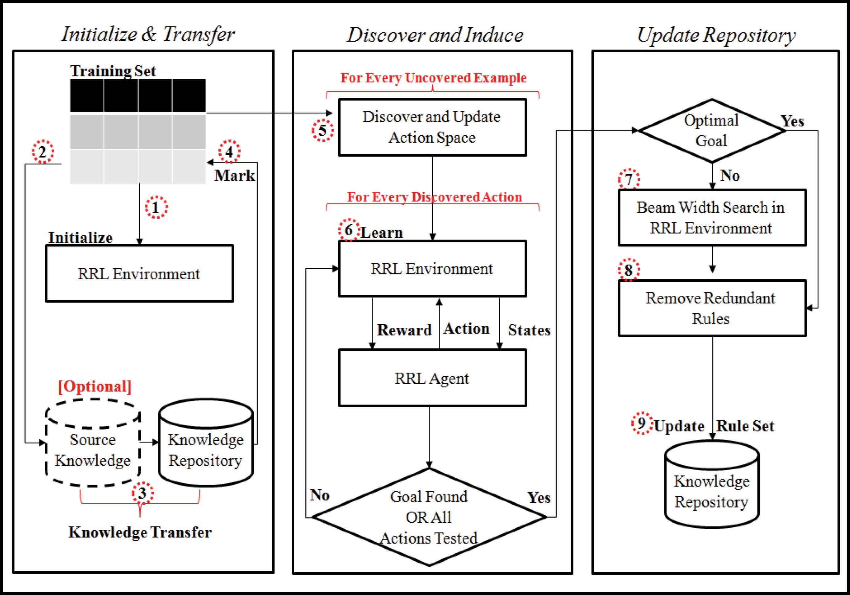
The basic idea of RULES-CONT is to address numeric features without discretization or fuzziness during rule induction. From Figure 2, RULES-CONT begins by reading the training set and initializing the parameters. In the first step, the initial RRL state space is defined to include the states that represent null rules for every class. In the second step, if the training set belongs to a previous patch of incremental examples, the incremental procedure is activated to transfer the agent’s previous knowledge, similarly to RULES-TL49, and flag examples in advance to reduce the search space. Hence, if there is a rule that cover a seed example (step 3), then that example is flagged as covered (step 4) and the rule is stored in the final rule set.
RULES-CONT learning approach
The RRL procedure is executed afterward (step 5 & 6) to discover new rules to flag uncovered examples. This search procedure addresses numeric values while discovering the best policy to represent the optimal rule. The search will proceed without prior assumptions for every seed such that all features are encompassed in a single state. When the goal state is found, it will be transformed into an if-then statement and applied to cover any matching examples. The details of this procedure will be explained later in section 4.2. The discovered rules are then stored in the final rule set. If the goal state has not yet been found (step 7), inconsistent rules that are near the goal will be selected as the final rule set using a beam width search. Finally, in step 8, identical rules are removed. The resulting rule set can then be used to classify future examples.
To understand how RULES-CONT manages numeric features, the details of the RRL environment and learning procedure are important. Therefore, in the following subsections, the RRL elements and technical details will first be explained, and the learning and prediction procedures will subsequently be presented.
4.1. RRL Elements and Environment
RRL elements need to be defined specifically for the numeric features problem. To understand how RRL is applied, this section presents the RRL elements for the CA problem for the agent to begin its learning.
4.1.1. RRL Environment
In RULES-CONT, the RRL environment is unknown and is built throughout the lifespan of the agent; the state space differs depending on the training set, and its actions change from one seed example to another to find the most appropriate value to cover the examples. This dynamicity is introduced to reduce the state and action spaces, in which only needed objects are stored. Moreover, because RRL is applied, a single state (rS) contains a number of states, and the same applies for the actions (rA). The algorithm searches for the most consistent state by applying different actions, and thus, different condition values (A ∈ rA) are added to obtain a consistent state rS with reward = 1.
4.1.2. rState Space
In RULES-CONT, each state contains several predicates that change based on its actions. The predicates represent all possible actions that can be applied over the features. These predicates are {Equal, Less, Greater, LessEqual, GreaterEqual} and are chosen to select the best alternatives for a feature value. The domain of these predicates includes the feature names and values. Note that predicates (or sub-states) containing either numeric or discrete values may be grouped together by the AND logical expression.
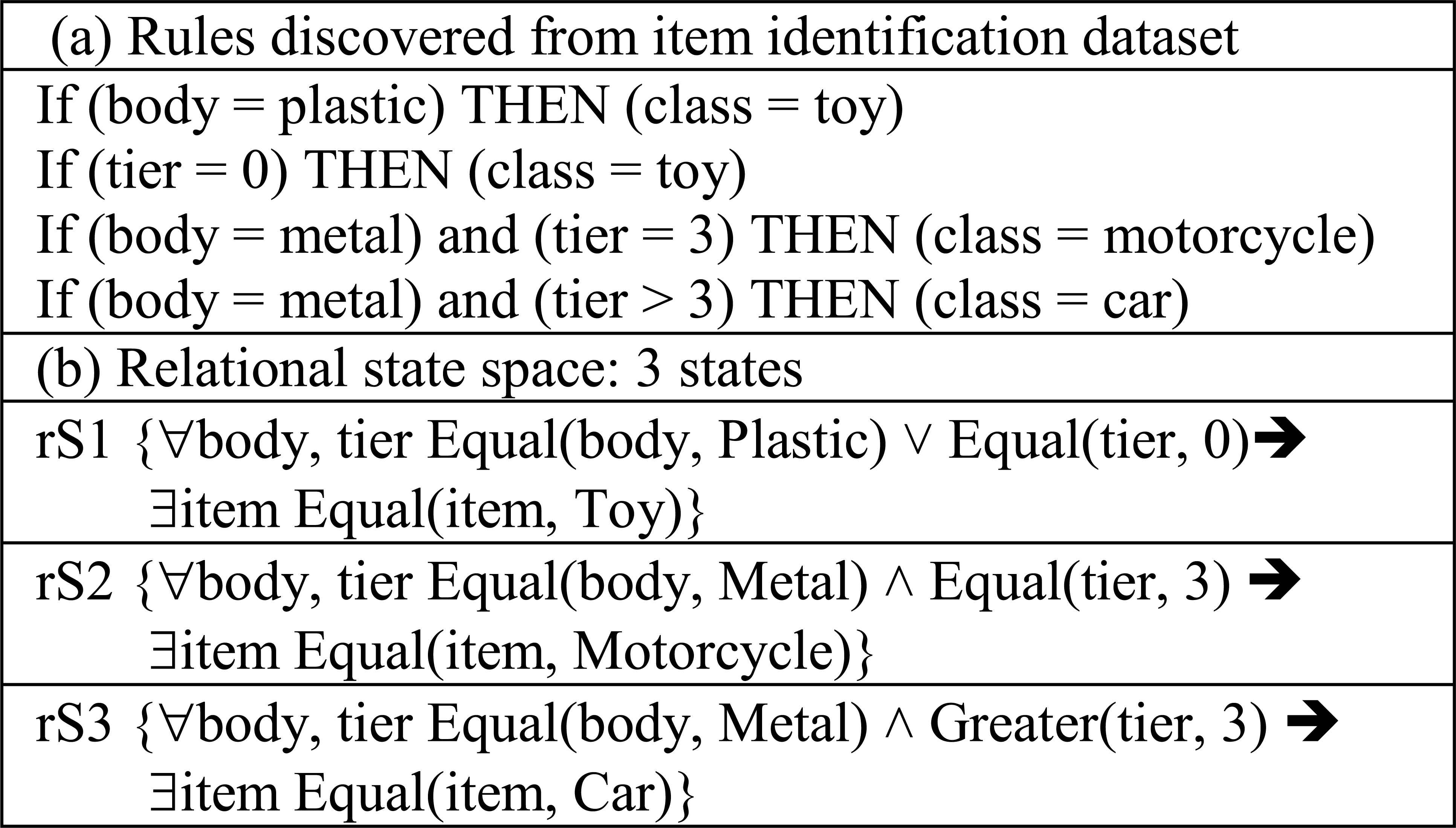
For example, Figure 3 shows the rules discovered from a dataset about item identification to demonstrate how RULES-CONT can represent these rules in the state space. In this dataset, an item can be identified as a toy, motorcycle, or car depending on its properties. Four discovered rules are presented in Figure 3.a, and RULES-CONT manages these rules as shown in Figure 3.b. If a new action {Less (tier, 5)} is discovered and added to rS3, then a new state { ∀body, tier Equal (body, Metal) ⋀ Greater (tier, 3) ⋀ Less (tier, 5) ➔ ∃item Equal(item, Car)} will be stored as rS4.
An example of an RRL state space in RULES-CONT containing three states
Note that the first and second rules are combined using OR because each contains only one feature; the NOT logical expression can also be added, depending on the technique used. Currently, RULES-CONT uses only the AND operation because it induces one rule at a time for each uncovered seed example. Moreover, it checks for conflicts and tests only actions that are applicable to the current state. For example, if the Equal (tier, 3) action is applied over rS3, then the predicate {Greater (tier, 3)} will be replaced to obtain a new state; the new action will not be added to rS3 because this predicate conflicts with the logical meaning of rS3.
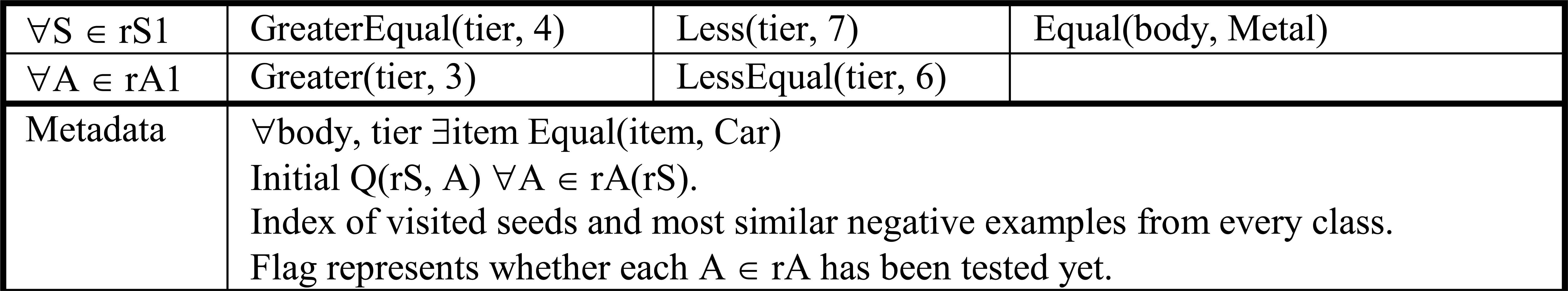
Every rS is associated with metadata to represent the logical meaning of the state and to indicate which seed example has visited the state, in addition to its most similar examples from every class. For example, the state { ∀body, tier Equal (body, Metal) ⋀ GreaterEqual(tier, 4) ⋀ Less(tier, 7) ➔ ∃item Equal(item, Car)} can be represented as shown in Figure 4. The action values for discrete features are the same as those for the seed, whereas the ranges for numeric features are created based on the most similar negative examples, as will be explained in the following sub-section.
An example of how state-space metadata are represented
4.1.3. rAction Space: Missing/Numeric Features
In RULES-CONT, both discrete and numeric features can be grouped together by logical operations. The sub-actions in every rA represent the possible values for every sub-state. For a feature (i), rA[i] represents the possible actions that can be assigned to one sub-state to transition to another state, regardless of that feature’s type. These actions are created based on the visited state and seed examples. Thus, the action space is also unknown and dynamic; it depends on the learning process. This increases the flexibility of the algorithm to address numeric features more accurately. In particular, when a seed example visits an rS, the most similar negative examples from every class are selected using (2), where the distance between discrete features is computed using (3). C and D are the lists of all numeric and discrete features of the data, respectively. ViE1 and ViE2 are the values of attribute (i) in examples E1 and E2, whereas Vimin and Vimax are the minimum and maximum values of feature (i). This measure, as explained by Pham et al.28, is a distance measure that can be used to compare any type of examples and all types of data.
After the most similar negative examples are selected, actions that belong to state rS are created from one of the cases presented in Figure 5. Note that Ei denotes feature i for the current seed example, Neg(i) denotes feature i for the most similar negative example, and the Min/Max functions return the minimum or maximum value of feature i from among all of the examples covered by the current state rS.
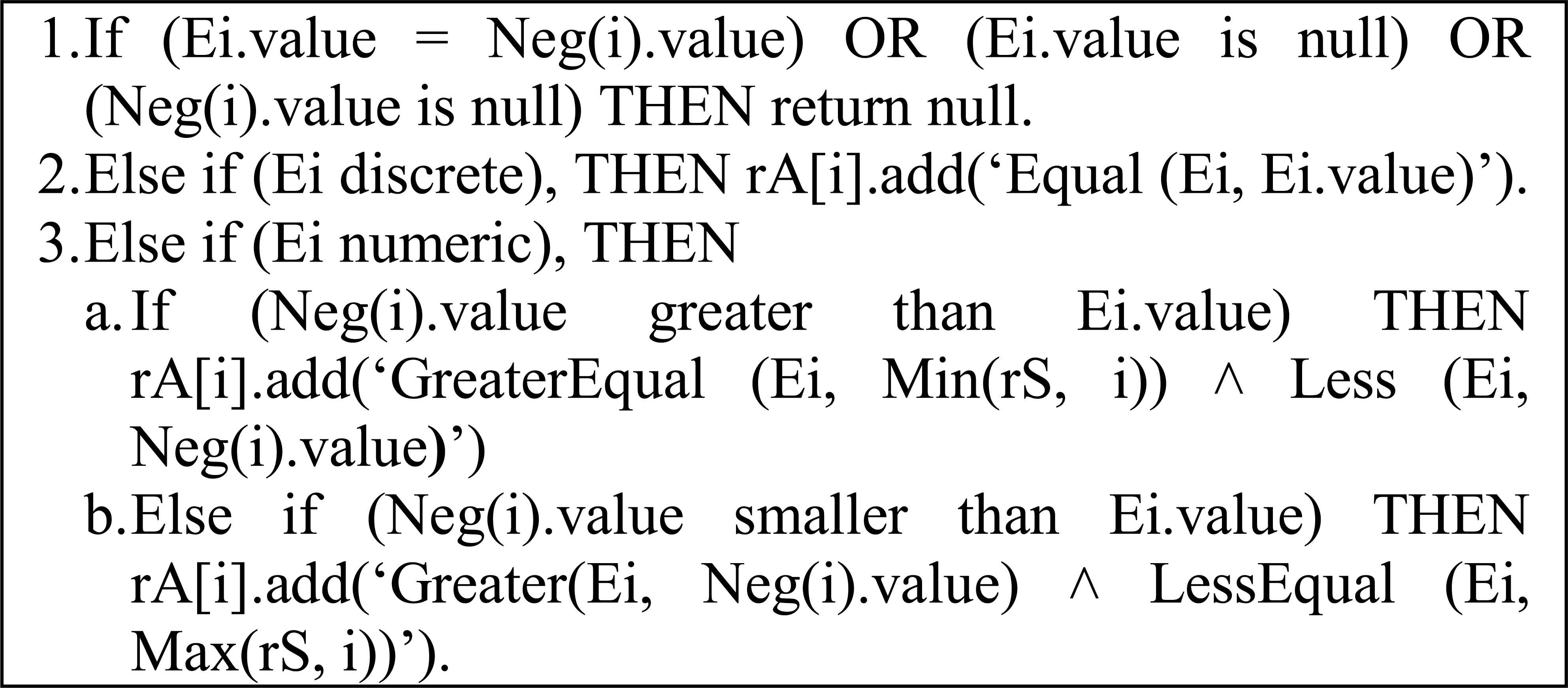
The rAction creation cases: (1) feature is empty, (2) feature is discrete, or (3) feature is numeric
As shown in Figure 5, the actions represent the possible values of numeric and discrete features. Through the RRL learning process, the best actions are chosen based on their Q values. To avoid discretization problems, fixed ranged are not applied; instead, new actions are created depending on the current seed. Moreover, as shown in step one in Figure 5, missing values are handled automatically by considering no actions for a missing value. The discovery of negative or overlapping rules is also avoided by neglecting identical negative examples. Note that the Q value of each discovered action is initialized to a non-zero value using (4), to start with the strongest actions. In equation (4), P(rA) is the number of positive examples (examples with values in the same range as action A), whereas E(rS) is the total number of examples covered by rS.
4.1.4. Rule Quality and Reward Function
In the RULES family, the rule quality is usually referred to as “search heuristics” and is used to automate the learning task.50 In IL, various measures can be applied to measure the quality of the discovered rules and to determine when rule learning should stop. These measures can be used to reduce excessive searching while preserving performance. For this purpose, various measures were tested with RULES-CONT, including the IREP value matrix51, the Hellinger measure52, the mestimate53, and the S-measure54. It was found that RRL handles numeric features more effectively when the rule consistency is monitored. Thus, the reward is computed using (5), where n is the number of negative examples covered by rS. The reward value lies in the interval [-1, 0] when the goal state has not yet been reached and becomes equal to one only upon reaching the goal.
By means of this reward function, RULES-CONT assigns the maximum penalty to null states to avoid rules with no conditions, which cannot be used in a classification model. The reward will be equal to one if the state does not cover any negative examples. In this case, the discovered rule is the desired one, and the search should stop. If the current state is neither the goal nor the null state, then the agent will be guided toward the goal based on the computed percentage of negative covered examples. A negative value is assigned because a rule that covers fewer negative examples is better. Thus, high rewards move the agent closer to the goal until n = 0 (i.e., r = 1).
4.1.5. Control Method
To apply RRL, a control method must be chosen to decide which action should be applied in a given state. One of the simplest and best-known control methods for RRL is called rQ-Learning18, 20, in which actions are repeatedly applied given the current state to learn a policy. When the agent visits a state, it selects an action based on a certain policy, such as the greedy policy. Then, the reward of the selected action is collected. Afterward, the action value is calculated in a greedy way, i.e., the optimal action value is selected. These steps are repeated until the stop condition is reached. The action value can be calculated using (6), where rS is the current state, rS’ is the new state, rA is the set of actions applied to transition from rS to rS’, r is the reward for applying rA over rS, and (0 ≤ α ≤ 1) and (0 ≤ γ ≤ 1) are the learning and discount factors, respectively. This equation is one of the simplest ways to compute the action value.55
4.1.6. Policy
In RULES-CONT, the optimal policy is that which discovers the most rewarding state within the fewest number of actions. Thus, the algorithm attempts to apply actions that will reach the goal state as rapidly as possible in the smallest number of steps. In general, every policy represents a rule, and the optimal one is the consistent rule with the fewest conditions.
4.1.7. Goal
The goal of RULES-CONT is to reach a consistent state with a reward equal to one. In this way, the discovered state can be translated into a rule that has overlapping conditions while avoiding conflict with other rules by virtue of its consistency. For example, if the goal state discovered is { ∀body, tier Equal(body, Metal) ⋀ Greater(tier, 3) ➔ ∃item Equal(item, Car)}, then this logical expression can be translated into the rule {If (Body = Metal) AND (Tier>3) THEN (Item = Car)}. This translation is possible because one of the main advantages of a CA is its ability to directly translate its discovered knowledge into any FOL expression.
4.2. RRL Learning Procedure
After building the initial RRL space and transferring knowledge of past rules, RULES-CONT initiates the RRL procedure to discover the best alternative values and induce the best rule for every uncovered example. As shown in Figure 6, to save computation time by starting from previously discovered states, the state rS with the highest reward that covers the current seed is chosen as the initial state. Then, the algorithm enters a loop in which it updates the environment and searches for the goal state. It does not stop until it finds the goal or when learning cannot be further improved. RULES-CONT attempts to avoid an exhaustive search by stopping the search even if the goal has not yet been found. Stopping the search in this way will not cause a problem in the future because it will later be possible to find the goal while iterating on a subsequent seed example using the knowledge extracted in a previous step. Thus, RULES-CONT might stop at a local minimum with the understanding that it will reach a global minimum in the future, instead of mistakenly regarding the local minimum as the global one.
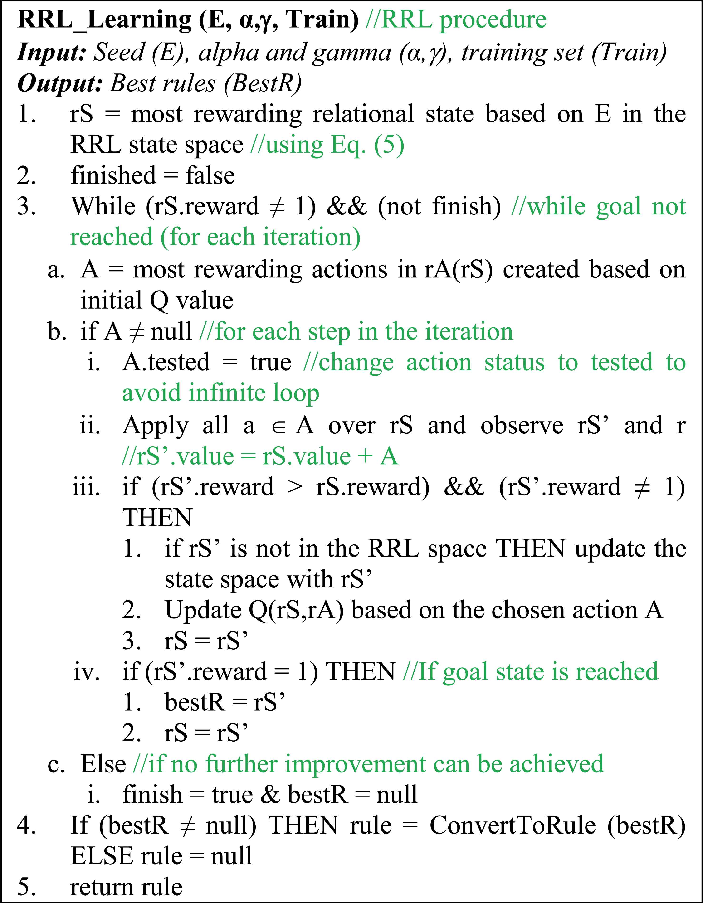
A Pseudo code illustrating how RRL is used to induce new rules from a numeric environment
In RULES-CONT, the RRL search begins with an update to the action space of the current state and the selection of the best action based on its strength (step 3.a). Based on the initial Q value defined in (4) and the actions’ reward, the best non-tested condition is chosen. Note that the score represents the reward obtained by adding an action A that belongs to rA to the incomplete state of rS, not the final expected rule. Thus, the algorithm operates on the current state to determine the best possible actions. In step 3.a, if a feature has a missing value, the RRL agent will automatically address it during action generation. If no actions are found or the actions of all features have already been tested at least once in the current state, then no further improvement can be achieved using the current state. In this case, the stop condition will be activated without the optimal rule being found, as stated in step 3.c. Note that the algorithm will not stop after testing only one action; instead, all features will be tested unless the goal is found beforehand. However, stopping the search at this point prevents an infinite loop.
When the stop condition is triggered without the goal state having been found, the local optimum discovered in this step will not be considered. Instead, the discovered information will be stored in the state space for later use. In this way, the global optimum can be sought while taking advantage of the information discovered throughout the lifespan of the RRL agent. When a new action is found, as in step 3.b, the algorithm first marks the action as tested. Then, the new state obtained after applying the action is observed, and its reward is computed. If the new state is better than the previous one but still is not the goal, then the algorithm updates the action value function of rS and continues to search for new states. The state space is also updated with the newly discovered state, as in step 3.b.iii. However, if the reward of the new state is equal to one (step 3.b.iv), then the goal has been reached and the search is stopped for the current seed.
Finally, after the goal state is found (step 4), the value of the goal state is converted into a rule represented as an ‘if-then’ statement instead of a logical expression. The best rule is then returned as the discovered rule. For example, a rule can be represented in the form {(A1, “K”) ^ (A2, (1,5]) ➔ (class, T)}. This string can be stored in the final rule set (knowledge repository) to be used for future predictions.
4.3. Prediction Procedure
After the best rules are discovered and the agent’s repository is produced, the resulting model should be used to predict classes. In RULES-CONT, three cases may arise when classifying an example, as follows:
- •
One Rule: When only one rule covers the example, this rule is used for prediction.
- •
No Rule: When no rules are found to match the example, the most similar rule is chosen based on its distance from the example. The distance between a rule and an example is computed using (7), (8), and (9), where C and D are the lists of all numeric and discrete features of the data, respectively. ViE and ViR are the values of feature (i) in example E and rule R, respectively; ViR.max and ViR.min are the maximum and minimum values, respectively, of the rule’s condition range; and Vimin and Vimax are the maximum and minimum values, respectively, of the numeric features in the training set. Note that if more than one rule has the same distance from the example, then the strongest one is used.
- •
Conflicting Rules: When multiple rules with different classes cover an example, the most similar rule is chosen to classify the example using (7).
5. Experiment
To assess the performance of the proposed algorithm, the KEEL tool was used to conduct 10-fold cross-validation experiments on a PC with a 2.40 GHz Intel® Core™ i7 CPU and 16 GB of RAM. First, the technical setup of the experiments in relation to RULES-CONT is presented. Then, the accuracies of RULES-CONT and seven other algorithms applied to datasets with numeric features are investigated at different levels of noise. Afterward, the total resistance level is visualized and the significance of the differences between the algorithms is statistically investigated using box plots and the Friedman test. Finally, the effect of the relational representation on the speed of RULES-CONT is discussed in comparison with its preceding version.
5.1. Experimental Setup
The experiment involved certain common elements that must be explained to understand the analysis details, including the parameters, algorithms, and dataset.
5.1.1. Algorithm Parameters
To initiate RULES-CONT, various parameters must be set to certain values. First, because a local beam search is applied when no solution is found, the beam width size was set to three. This value is the default value that has been found to be appropriate for the RULES family. Second, the RRL parameters (alpha α and gamma γ) were initialized to 0.5 based on the standard proposed by Sutton and Barto55, in which equal weights are assigned to past and current knowledge.
5.1.2. Comparative Algorithms
To demonstrate the improvement in rule induction performance achieved by RULES-CONT, it was compared with seven other algorithms, as follows:
- •
RULES-5+: A fuzzy non-discretization RULES algorithm that uses incremental post-pruning (IPP) when noise is present in the data.
- •
- •
Slipper and Ripper: Algorithms from the REP-based family that use reduce-error pruning. They handle numeric values using online discretization. Slipper, however, incorporates ensemble learning to address conflicts.
- •
C4.5RulesSA58: An extended version of C4.5 that transfers knowledge from the decision tree into rules. It uses simulated annealing to search for the best split points during induction and applies back pruning to remove weak branches.
- •
DT_GA: A hybrid decision tree algorithm that handles numeric values online during rule induction using a genetic algorithm. An information-theory-based pruning technique is applied to reduce the number of conditions and achieve early termination.
5.1.3. Dataset
To demonstrate the reliability of the proposed algorithm, it was tested on 27 datasets. These datasets were drawn from the KEEL dataset repository and gathered as real-life samples. Each dataset has its own characteristics, as summarized in Table 2.
| Name | #Examples | #Features | #Classes |
|---|---|---|---|
| Balance | 625 | 4 | 3 |
| Contraceptive | 1473 | 9 | 3 |
| Ecoli | 336 | 7 | 8 |
| Solar Flare | 1066 | 11 | 2 |
| Glass | 214 | 9 | 7 |
| Heart | 270 | 13 | 2 |
| Ionosphere | 351 | 33 | 2 |
| Iris | 150 | 4 | 3 |
| Led7digit | 500 | 7 | 10 |
| Newthyroid | 215 | 5 | 3 |
| Nursery | 12960 | 8 | 5 |
| Page-blocks | 5473 | 10 | 5 |
| Penbase | 10992 | 16 | 10 |
| Pima | 768 | 8 | 2 |
| Ringnorm | 7400 | 20 | 2 |
| Satimage | 6435 | 36 | 7 |
| Segment | 2310 | 19 | 7 |
| Shuttle | 58000 | 9 | 7 |
| Sonar | 208 | 60 | 2 |
| Spambase | 4597 | 57 | 2 |
| Splice | 3190 | 60 | 3 |
| Thyroid | 7200 | 21 | 3 |
| Twonorm | 7400 | 20 | 2 |
| Vowel | 990 | 13 | 11 |
| WDBC | 569 | 30 | 2 |
| Yeast | 1484 | 8 | 10 |
| Zoo | 101 | 17 | 7 |
The benchmark dataset properties
Dataset properties can affect the algorithm performance. Thus, it was decided to characterize the datasets based on the results of the algorithms. Specifically, a dataset with fewer than 1000 instances is considered to have a small number of examples, between 1000 and 10,000 is considered a medium number of examples, more than or equal to 10,000 and fewer than 40,000 instance is considered a large number of examples, and more than or equal to 40,000 is considered a very large number of examples. Moreover, a number of features less than or equal to 10 is small, between 10 and 20 is a medium number of features, more than or equal to 20 and fewer than 40 is a large number of features, and more than or equal to 40 is a very large number of features. Finally, a number of classes less than or equal to 5 is small, between 5 and 10 is a medium number of classes, and more than 10 is a large number of classes. Although in general, large datasets typically contain millions of examples, these characteristics were chosen for differentiating the algorithms’ performance based on the sampled datasets.
5.2. Accuracy Investigation
This section considers the algorithms’ behavior at different levels of noise and compares their performance in the absence of noise. In particular, four levels of noise were introduced into the datasets from the KEEL repository59: 0%, 5%, 10%, and 20%. The accuracy of the algorithms was compared based on their error rates on every dataset. RULES-CONT does not include any pruning technique since it was developed to be able to accurately predict the classes of numeric and noisy data while avoiding the need to apply additional techniques.
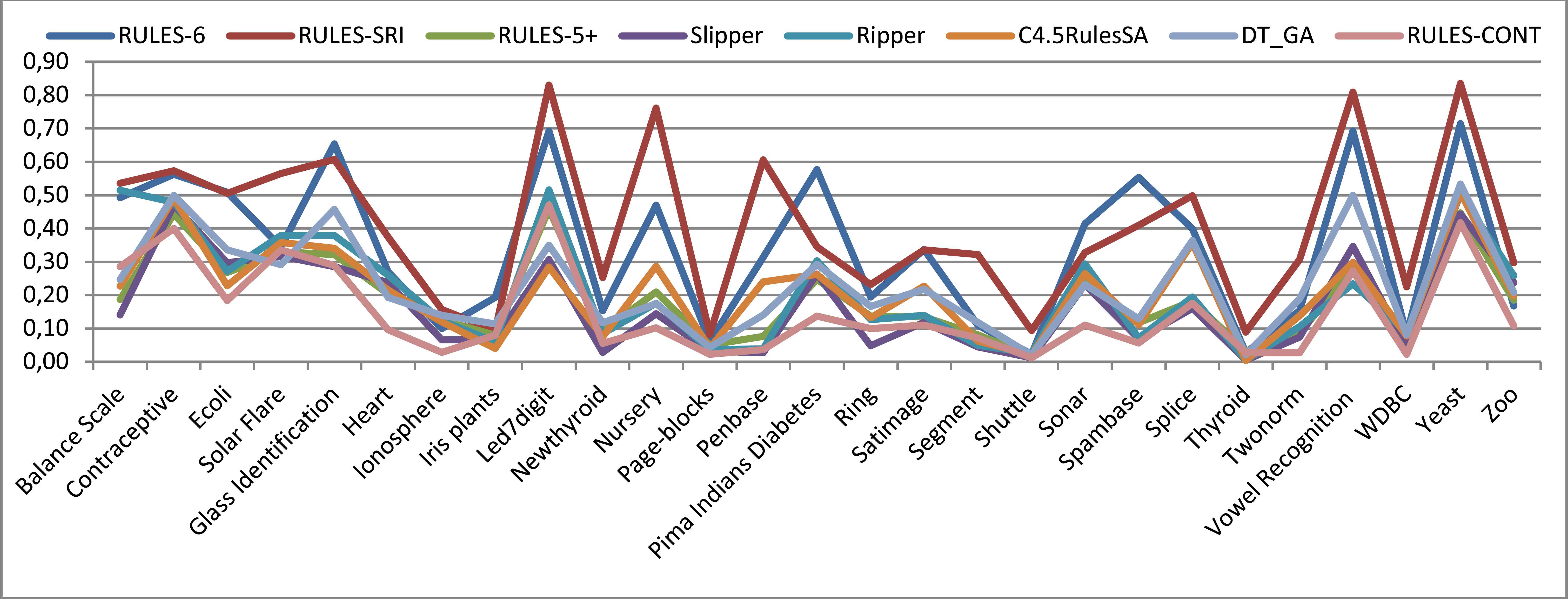
At 0% noise (Figure 7), RULES-CONT exhibits the smallest error rate on most datasets. However, its performance suffers for datasets that contain large numbers of examples and features but a small number of classes, such as the Splice and Solar Flare datasets; it is also outperformed by other algorithms on datasets with a large number of classes that contain relatively few examples and features, such as the Led7digit dataset. The accuracy of RULES-CONT, in general, is similar to that of RULES-5+. The online-discretization-based algorithms, including Slipper, Ripper, DT_GA, and C4.5RulesSA, yield the next best error rates, and the offline-discretization-based algorithms give the least accurate results. Hence, the following conclusion can be stated:
Conclusion #1: Addressing numeric features using a non-discretization approach yields the most accurate results, followed by online discretization and then offline discretization-based algorithms.

Error rates obtained in 10-fold cross-validation with 0% noise
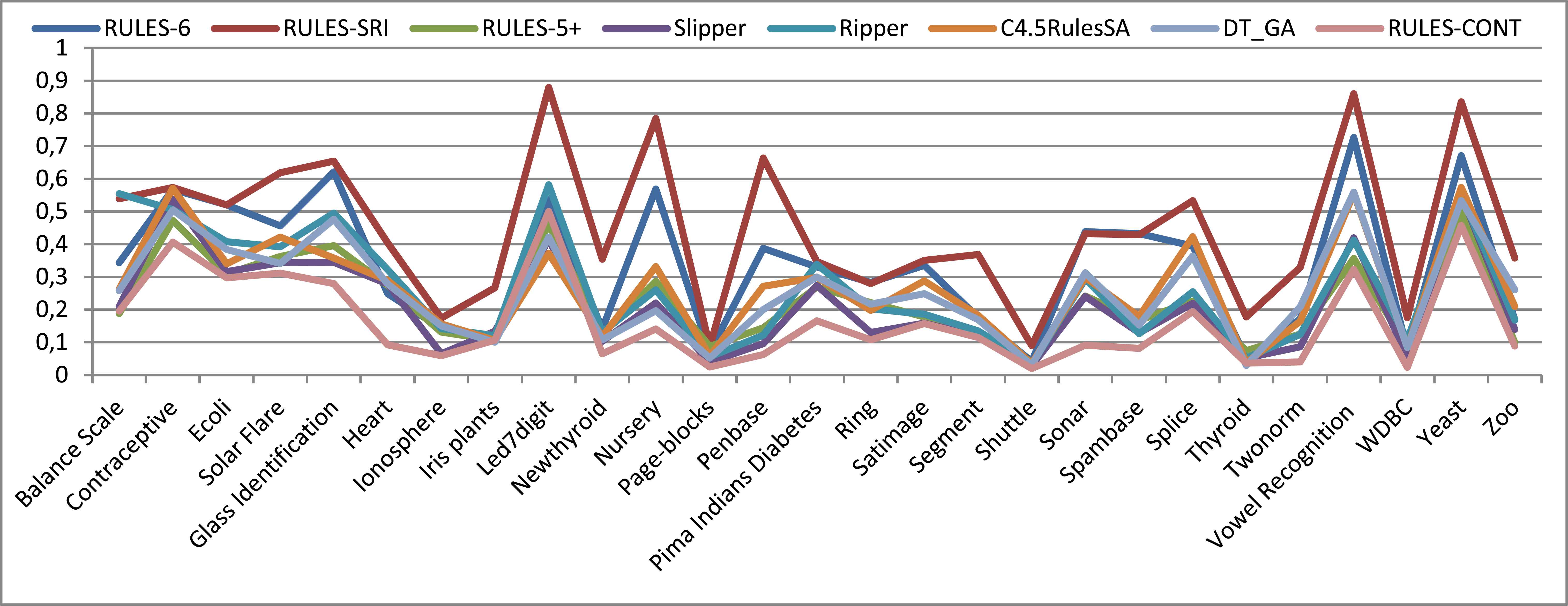
When 5% noise is introduced (Figure 8), the behavior of the algorithms changes accordingly. From the figure, it is apparent that the accuracy of RULES-5+ is more affected by the noise than is that of RULES-CONT or Slipper. RULES-CONT remains the most accurate, but its performance becomes more similar to that of Slipper than that of RULES-5+, indicating that it is more resistant to noise than is its preceding version in the family. When the dataset properties are considered, it appears that RULES-CONT is more resistant to noise when the numbers of examples and features are large than when the number of classes is large. The other algorithms are also affected by the presence of noise; all of them exhibit increases in error rate, except for RULES-6. This algorithm maintains similar performance to that achieved on non-noisy data; however, considering that its performance was poor from the start, this resistance is not particularly beneficial. It sacrifices its current accuracy for increased variance and resistance to future noise. In fact, RULES-CONT and RULES-6 are the most noise-resistant algorithms, but whereas the former exhibits the best accuracy, the accuracy of the second is the worst. The conclusion yielded by these observations can be summarized as follows:
Conclusion #2: Unlike the preceding offline-discretization-based algorithm in the same family, RULES-CONT achieves both current and future accuracy in a noisy environment rather than sacrificing one for the other.
Error rates obtained in 10-fold cross-validation with 5% noise
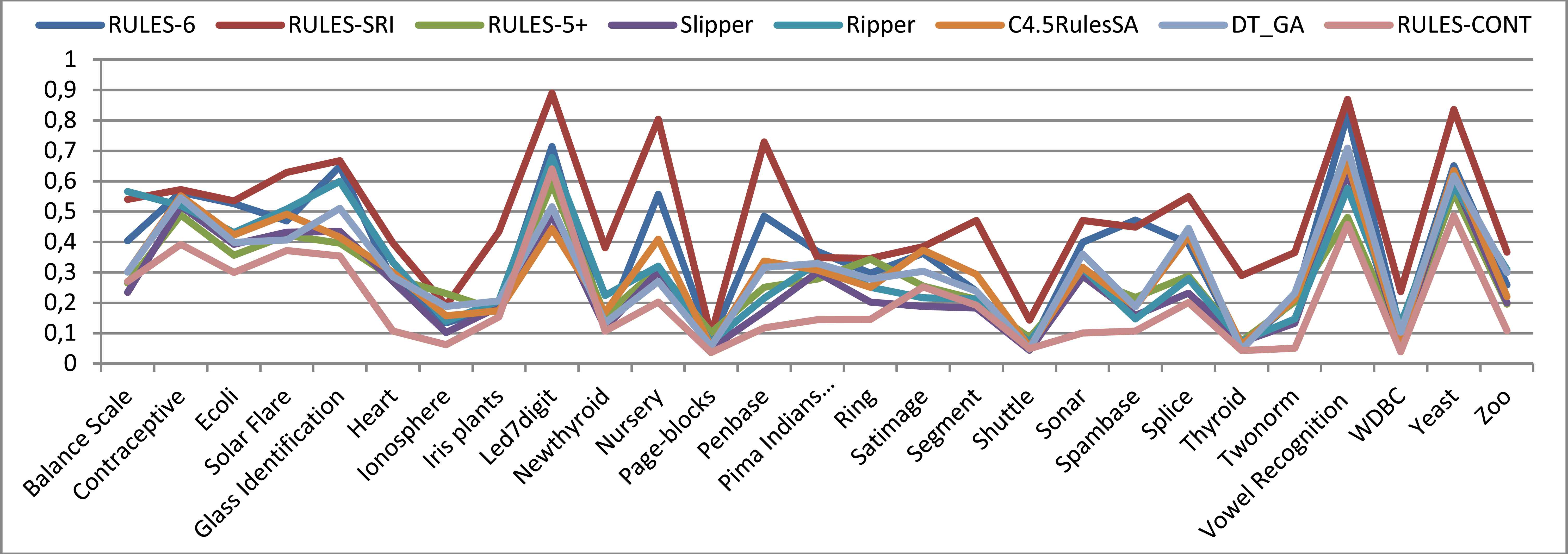
Upon an increase in the noise to 10% (Figure 9), RULES-CONT retains its ranking with respect to the other algorithms, producing the lowest error rates on most datasets, while RULES-6 and RULES-SRI continue to exhibit the worst error rates on most datasets. Whereas the error rate of RULE-SRI increases with increasing noise, RULES-6 maintains a similar accuracy, indicating that RULES-6 is more resistant to noise than is RULES-SRI. The gap between RULES-6 and the other algorithms, with the exception of RULES-CONT, decreases with an increasing noise percentage. Hence, increasing the noise percentage increases the error rates of both online and previous non-discretization-based algorithms, indicating that these algorithms sacrifice their future accuracy for current accuracy. By contrast, even as the level of noise in the data increases, the effect on RULES-CONT is less severe than the effect on the other algorithms. With an increasing level of noise, RULES-CONT becomes the best-performing algorithm for almost all datasets. Its accuracy is obviously affected only on the Led7digit dataset, which contains small numbers of examples and features but a large number of classes. This is because the dataset does not provide sufficient information about the problem but requires predictions for a large number of classes. Based on these observations, the following conclusion can be stated:
Conclusion #3: The implementation of RRL in the RULES family increases noise resistance while allowing numeric features to be accurately addressed without the need for discretization or complex fuzzy theory.
Error rates obtained in 10-fold cross-validation with 10% noise
To ensure that RULES-CONT can maintain this behavior even as the noise is further increased, another test was conducted with 20% noise. Figure 10 shows that the error rate of RULES-6 does not significantly change upon increasing the noise percentage to this level. The error rates of the other algorithms, except for RULES-CONT, shift away from that of RULES-CONT and become more similar to that of RULES-6 when the noise is increased to 20%. By contrast, the behavior of RULES-CONT in terms of accuracy remains similar to that at 10% noise; its error rate is still obviously higher than those of several other algorithms on Led7digit, and a slight increase is also observed on the Satimage dataset. Therefore, RULES-CONT is less affected by an increase in noise than are the other algorithms. Consequently, the following conclusion can be stated:
Conclusion #4: Although RULES-CONT does not apply any special pruning technique, it achieves the best performance at all levels of noise.
Error rates obtained in 10-fold cross-validation with 20% noise
All of the above results clearly demonstrate the noise resistance achieved by using RRL. However, it is also important to statistically study the significance of the differences between the algorithms. The following section presents such an analysis and visualizes the behavior of the algorithms in all noise cases.
5.3. Noise Resistance
In addition to the accuracy, it is also important to measure to what extent each algorithm can resist noise. Therefore, this section presents visualizations of the accuracy of the algorithms to present the total resistance level of all algorithms. The Friedman test is also applied to demonstrate that the difference in error rate becomes more significant as the noise level increases.
5.3.1. Overall Resistance Level
To visualize and confirm the overall noise resistance of RULES-CONT, box plots were constructed to represent the error rate results, as shown in Figure 11. In this plot, the boxes represent the distributions of the results for each algorithm. The different algorithms are represented on the X axis, and the error rate is displayed on the Y axis. For each algorithm, the “+” sign indicates the mean of the results, the horizontal line inside each box represents the median, and the vertical lines above and below the boxes point to the maximum and minimum values. Note that outliers are represented by dots and that the two areas inside the box represent the upper quartile (above the median) and the lower quartile (below the median). From this visualization, it is possible to understand the distribution of the results and to compare the algorithms total noise resistance.
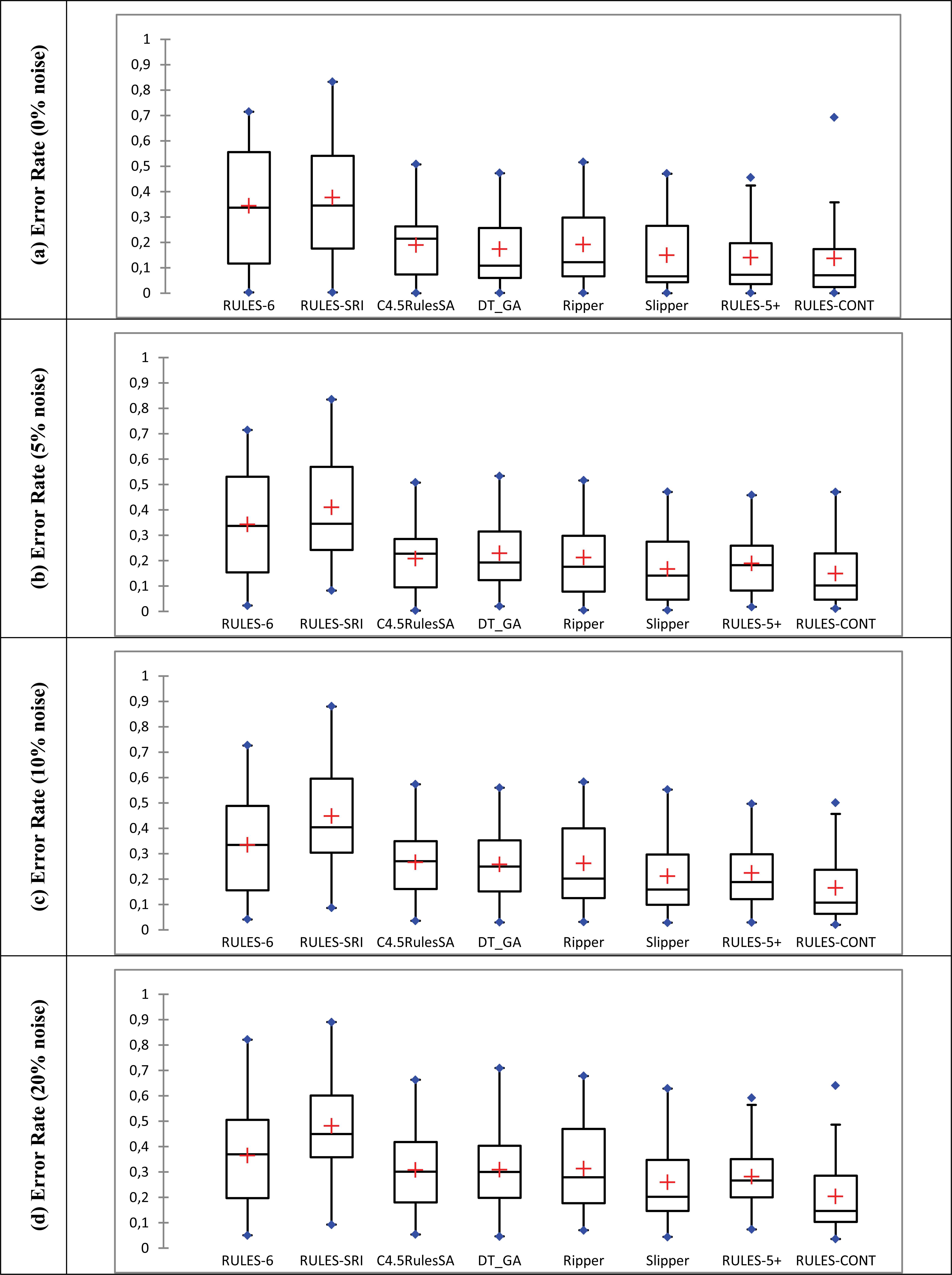
Box plots representing the error rates for all algorithms over all folds in all datasets
From Figure 11, it is clear that in all four cases, RULES-6 and RULES-CONT are the best to resist noise, as the locations of their boxes do not visibly change. However, as indicated by the fact that the box for RULES-6 is located higher than that for RULES-CONT and represents a larger range of results, the accuracy of RULES-6 is very low in comparison with that of RULES-CONT. Therefore, these two algorithms can be used as references to analyze the behavior of the other algorithms. In particular, when the box plot of an algorithm is seen to approach that of RULES-6 with increasing noise, it can be said to have low resistance and to suffer from a worsening error rate with increasing noise. By contrast, if the box plot approaches that of RULES-CONT with increasing noise, this algorithm can be said to resist noise and to be accurate even when noise is introduced.
Unfortunately, however, the plots for all algorithms considered here begin to approach that of RULES-6 with increasing noise, with their boxes moving upward in the graphs. In the absence of noise (Figure 11.a), RULES-CONT already exhibits the lowest error rate compared with the other algorithms. Even the value of the high-error outlier is still less than the maximum values for RULES-6 and RULES-SRI. In fact, this outlier is helpful for generalizing the results of RULES-CONT to future cases. A comparison of RULES-CONT with the other algorithms reveals that the mean and median error rates for this algorithm are almost identical to those for RULES-5+ and Slipper. These three algorithms appear to be the best when comparing the positions of their boxes with the others.
However, when considering the upper and lower quartiles of RULES-CONT with RULES-5+ and Slipper, it is clear that RULES-CONT is superior. The upper quartile of RULES-CONT ends at 0.15, whereas that of RULES-5+ ends at 0.19 and that of Slipper ends at 0.29. Moreover, 30% of the RULES-CONT results lie below the median line, whereas only 25% and 10% of the results lie below the median for RULES-5+ and Slipper, respectively. Finally, RULES-CONT has the lowest maximum value among the three algorithms. All of these findings confirm that the use of RRL improves the accuracy when applied to numeric features dataset.
In addition to the accuracy of RULES-CONT, its noise resistance should also be studied based on Figure 11. At all levels of noise (Figure 11.b, c, d), the RULES-CONT box remains lower than the rest, and the minimum and maximum values are also lower than those for the other algorithms. Upon an increase in the noise level, the boxes for all algorithms (except for RULES-6 and RULES-CONT) begin to move upward, indicating that the error increases exponentially with increasing noise. This effect is especially obvious for the non-discretization algorithm RULES-5+ because of its high overfitting of the data.
With regard to the mean and median error rates, RULES-CONT has the lowest values at all non-zero levels of noise. In the presence of noise, the minimum error rate for RULES-CONT becomes lower than those for the others, even though the minimum error rates of several of the algorithms are equally low in the absence of noise. Moreover, RULES-CONT maintains approximately the same distribution of error rates, in which 25% of the results lie below the median. Finally, the median error rate for RULES-CONT actually decreases with increasing noise, again indicating its superiority compared with the other algorithms. All of these findings confirm that RULES-CONT exhibits better overall noise resistance while guaranteeing better accuracy, even in the absence of noise.
In addition to the box plots, to compare the total performance of the algorithms over all datasets, the total error rate for each algorithm is summarized in Table 3. The last row represents the variance increase in the error rate to show how much the error rate increased in total. This table shows that RULES-6 is almost unaffected by noise, as the difference between the minimum and maximum error rates is only 3%. However, its lowest total error rate is still the worst after that of RULESSRI. Although it is not affected by noise, its accuracy in general is insufficient, as it produces a high error rate even in the absence of noise. RULES-CONT exhibits the next best noise resistance after RULES-6, with a difference in error rate of only 6%. Thus, its performance is not strongly affected by the noise level. In particular, the difference between the changes in error rate for RULES-CONT and RULES-6 is 3%, and at each noise level, the difference between the error rates of these two algorithms is higher than their differences from the others.
| Noise level | CONT | RULES-6 | SRI | RULES-5+ | Slipper | Ripper | C4.5RulesSA | DT_GA |
|---|---|---|---|---|---|---|---|---|
| 0% | 0.14 | 0.34 | 0.38 | 0.14 | 0.15 | 0.19 | 0.19 | 0.17 |
| 5% | 0.15 | 0.34 | 0.41 | 0.19 | 0.17 | 0.21 | 0.21 | 0.23 |
| 10% | 0.16 | 0.33 | 0.45 | 0.22 | 0.21 | 0.26 | 0.27 | 0.26 |
| 20% | 0.20 | 0.36 | 0.48 | 0.28 | 0.26 | 0.31 | 0.31 | 0.31 |
| Min-Max% | 6% | 3% | 10% | 14% | 11% | 12% | 12% | 14% |
Total error rates at different noise levels
Compared with the other algorithms, RULES-CONT generalizes better. When the noise level was increased from 0% to 20%, the error rates increased by 10% for RULES-SRI, 14% for RULES-5+, 11% for Slipper, 12% for Ripper, 12% for C4.5RulesSA, and 14% for DT_GA. Moreover, the results at every level indicate that RULES-CONT always exhibits the best performance. It produces the lowest error rate at all levels of noise, with results equal to those of RULES-5+ at 0% noise. At every noise increment, the increase in the error rate is smaller for RULES-CONT than for the other algorithms. Consequently, even though pruning is not applied in this algorithm, RULES-CONT is still superior. Based on all of these observations, the following conclusion can be stated:
Conclusion #5: RULES family with offline discretization is resistant to noise, but introducing RRL into the family improves its noise resistance and accuracy without the need for discretization.
5.3.2. Resistance Significance
To determine whether the improvement in noise resistance offered by RULES-CONT is significant, the statistical method proposed by Demsar60 was applied. For all datasets, the results of all algorithms were statistically compared using the XLSTAT tool61. Following the Friedman test, the Nemenyi post hoc test was also applied, and the results are presented as CD diagrams in Figure 12. Such a diagram represents the significance of the differences between the algorithms, where the numbers on the vertical lines indicate the rank and the thick lines indicate the groups, whereas the CD line indicates the algorithms that exhibit a significant difference from RULES-CONT.
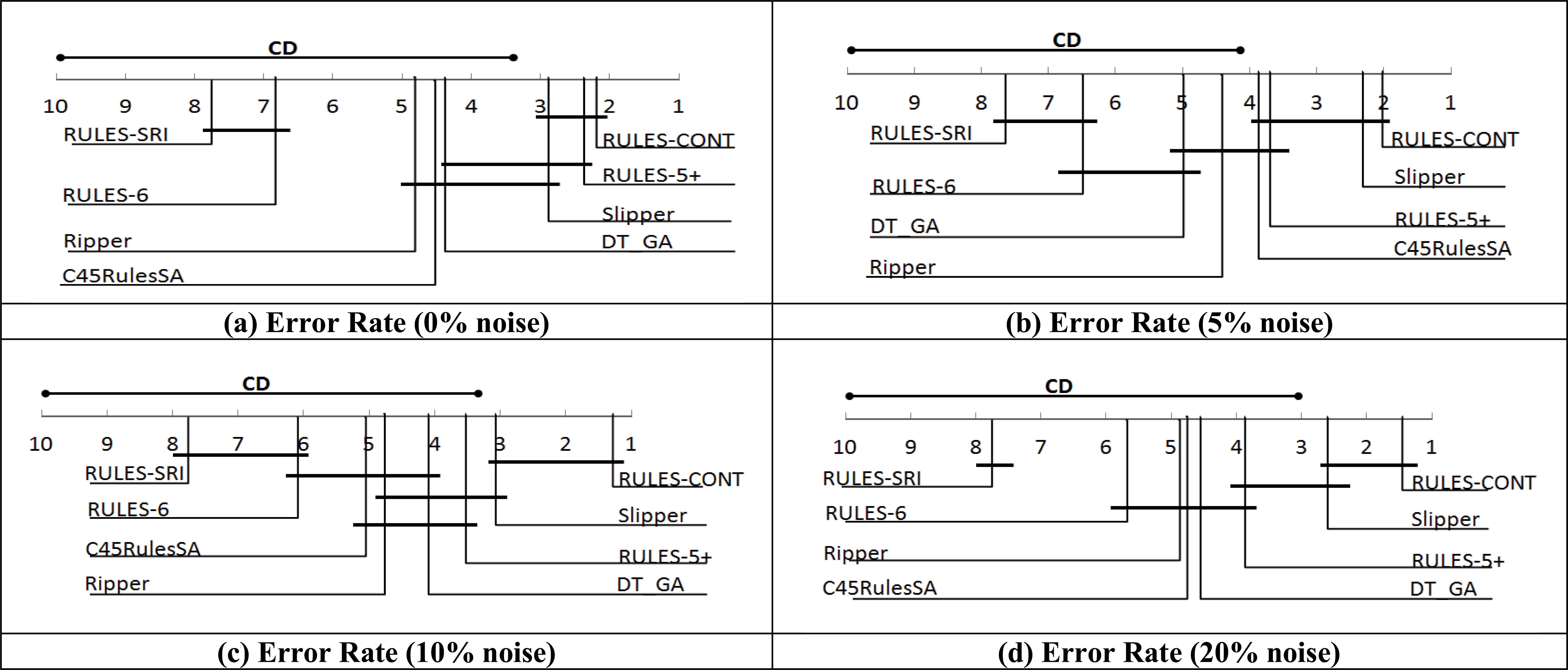
CD diagrams of the two-tailed Nemenyi post hoc test for all algorithms over all folds in all datasets
As shown in Figure 12, RULES-CONT is superior to the other algorithms at all levels of noise. It remains highest ranked while the other algorithms decrease in accuracy with increasing noise. At all noise levels, RULES-SRI is ranked lowest, with a rank of approximately 7.7. Its rank does not change, indicating that it performs the same in all cases compared with the other algorithms. By contrast, RULES-CONT is ranked highest at all levels, but its rank in each case is better than in the previous one, indicating that its performance improves compared to the others when increasing noise. Therefore, it can be concluded that the error rates of most algorithms worsen with increasing noise, whereas RULES-CONT is minimally affected by noise.
In more detail, when there is no noise (Figure 12.a), RULES-CONT is ranked highest, with an accuracy similar to those of Slipper and RULES-5+ and significantly better than those of the other algorithms. Algorithms that take a non-discretization approach typically perform better on datasets with numeric features. However, this no longer holds once noise is introduced (Figure 12.b). In this case, RULES-5+ performs worse than Slipper, indicating that the previous non-discretization algorithm in the RULES family has difficulties with noisy data because it overfits its training set. However, introducing RRL has solved this problem, and RULES-CONT remains highest ranked when 5% noise is introduced. It shows an insignificant difference from Slipper, RULES-5+, and C4.5RulesSA and a significant difference with respect to the others.
With increasing noise, however, the significance results change. When 10% noise or more is introduced (Figure 12.c and d), the error rate of RULES-CONT becomes significantly better than those of all other algorithms and similar to that of Slipper. It has the highest rank for both 10% and 20% noise. The performance of RULES-5+, meanwhile, further degrades with increasing noise, indicating that RRL is indeed a good solution for handling numeric data and predicting actions based on the rules induced from such data. Consequently, RULES-CONT is superior to other versions of RULES for addressing noisy and numeric data.
5.4. Process Time
In RULES-CONT, the time consumption of the algorithm is reduced through the use of the relational representation and re-use of past experience. However, this claim must be verified; thus, the effect of incorporating RRL on the speed of the algorithm must be investigated in addition to the effects on accuracy and noise resistance. This section presents an analysis of the process time of RULES-CONT and compares it with that of the preceding non-discretization RULES algorithm without relational representation (RULES-5+) to focus on the effect of the relational representation and the difference in speed with and without RRL.
Figure 13 shows the process times of the RULES-CONT and RULES-5+ algorithms at all levels of noise. From all graphs, it is evident that the speeds of RULES-CONT and RULES-5+ are similar, except on medium to large datasets with a non-small number of attributes. In particular, when the noise level is 0% (Figure 13.a) or 5% (Figure 13.b), the speed of RULES-CONT is slightly better than that of RULES-5+ on the Penbase dataset and significantly better on the Ring, Spambase, and Twonorm datasets. However, on the Satimage and Segment datasets, RULES-CONT is slightly slower than RULES-5+. This increase in speed is due to the dataset properties, as the Satimage and Segment datasets include not only medium to large numbers of examples and attributes but also a medium number of classes.

The process time for RULES-CONT and RULES-5+ at four levels of noise
When the noise increases to 10% (Figure 13.c) or 20% (Figure 13.d), RULES-CONT and RULES-5+ again have similar process times; except on medium to large datasets with a non-small number of attributes. However, the RULES-CONT process time decreases further compared with that of RULES-5+. In particular, the RULES-CONT process time becomes less than that of RULES-5+ on the Satimage and Segment datasets and noticeably better on the Penbase dataset. Hence, an increase in the level of noise has less effect on RULES-CONT speed than on RULES-5+.
Ultimately, when the speeds are compared at all levels of noise, the difference between RULES-CONT and RULES-5+ increases with increasing noise. On the Penbase dataset, the speed of RULES-CONT is only slightly lower than that of RULES-5+ at 0% noise, but the difference increases with increasing noise such that this difference is clear to the naked eye at 20% noise. On the Satimage and Segment datasets, at 0% noise, RULES-CONT is slightly slower than RULES-5+, but it becomes faster than RULES-5+ with increasing noise. The relational representation therefore improves the speed of RULES-CONT, and noise has a greater effect on RULES-5+, despite the fact that RULES-CONT does not prune and RULES-5+ does. All observations on the process time can be summarized as follows:
Conclusion #6: Introducing RRL into the RULES family reduces the time required to process noisy and numeric data without the need for any special pruning technique.
6. Discussion
RULES-CONT has the ability to learn from scratch and to re-use previously gathered knowledge to improve its rule selection behavior. Because it uses the relational representation, the algorithm can address multiple features and values as a single entity, and missing values are automatically handled when constructing actions. RULES-CONT cumulatively learns throughout its lifetime because one of the fundamental properties of RRL is continuous learning. Hence, incremental learning can be easily integrated with this method. The history of the RRL agent is preserved during rule induction; hence, it does not always need to start from a null state but instead can start from previously discovered ones. RULES-CONT temporarily stops its search when the goal cannot be found for any reason. However, once another seed example is discovered, the algorithm continues its learning while taking advantage of its past experience. Hence, it will sometimes stop at a local minimum with the intent of reaching a global one.
From the practical tests, it was concluded that RULES-CONT resolves the noise tolerance problem recognized in the literature while also offering improved accuracy. In particular, the following conclusions can be drawn regarding RULES-CONT:
- •
Handling numeric features using a non-discretization approach yields the most accurate results.
- •
RULES-CONT preserves both its current and future accuracy and does not sacrifice one for the other.
- •
The use of RRL in the RULES family increases noise resistance while allowing numeric features to be accurately addressed without discretization.
- •
According to the Friedman test, RULES-CONT maintains the highest ranking among comparable algorithms at all levels of noise.
- •
Introducing the relational representation into the RULES family improves the speed and decreases the effect of noise even when pruning is not applied.
Addressing infinite-space values using a non-discretization approach that continuously learns from experience can improve the performance of CAs. RULES-CONT incorporates new properties into a CA but also offers improved accuracy and noise resistance. Updating the resulting quantization does not pose a problem because the ranges for numeric features are not fixed but rather are handled dynamically. RULES-CONT does not suffer any trade-off in performance to accurately address infinite-space values; instead, it offers improved accuracy while also maintaining high noise resistance.
7. Conclusion
This paper introduced a novel non-discretization approach based on RRL. This approach was used to develop an algorithm called RULES-CONT, which addresses both numeric and discrete values in a similar manner and attempts to discover the best values for a set of features as a whole depending on their common characteristics and their relationships with other examples and classes. The results of experiments and statistical tests verified that RULES-CONT fills the existing performance gaps of CAs. It offers improved accuracy and speed for a CA while maintaining a high level of noise resistance. The problems faced by discretization methods are avoided because it uses a non-discretization approach. In the future, the effects of pruning will be tested to compare the behavior of RULES-CONT with that of other algorithms that apply pruning. Additional logical expressions will also be integrated to further scale the algorithm; for example, the NOT and OR operations can be used to group several states together and thus reduce the space to enable the processing of terabyte datasets.
Acknowledgments -
This research project was supported by a grant from King Abdulaziz City for Science & Technology. We also thank Dr. Samuel Bigot for his cooperation in providing us with RULES-5+.
Footnotes
Through this document, the term ‘numeric’ corresponds to numeric and continuous values.
References
Cite this article
TY  - JOUR
AU  - Hebah ElGibreen
AU  - Mehmet Sabih Aksoy
PY  - 2016
DA  - 2016/06/01
TI  - Adopting Relational Reinforcement Learning in Covering Algorithms for Numeric and Noisy Environments
JO  - International Journal of Computational Intelligence Systems
SP  - 572
EP  - 594
VL  - 9
IS  - 3
SN  - 1875-6883
UR  - https://doi.org/10.1080/18756891.2016.1175819
DO  - 10.1080/18756891.2016.1175819
ID  - ElGibreen2016
ER  -