
An Efficient Artificial Fish Swarm Model with Estimation of Distribution for Flexible Job Shop Scheduling
- DOI
- 10.1080/18756891.2016.1237190How to use a DOI?
- Keywords
- Flexible job shop scheduling; artificial fish swarm model; estimation of distribution; Friedman test and Holm procedure
- Abstract
The flexible job shop scheduling problem (FJSP) is one of the most important problems in the field of production scheduling, which is the abstract of some practical production processes. It is a complex combinatorial optimization problem due to the consideration of both machine assignment and operation sequence. In this paper, an efficient artificial fish swarm model with estimation of distribution (AFSA-ED) is proposed for the FJSP with the objective of minimizing the makespan. Firstly, a pre-principle and a post-principle arranging mechanism that operate by adjusting machine assignment and operation sequence with different orders are designed to enhance the diversity of population. Following this, the population is divided into two sub-populations and then two arranging mechanisms are applied. In AFSA-ED, a preying behavior based on estimation of distribution is proposed to improve the performance of algorithm. Moreover, an attracting behavior is proposed to improve the global exploration ability and a public factor based critical path search strategy is proposed to enhance the local exploitation ability. Simulated experiments are carried on BRdata, BCdata and HUdata benchmark sets. The computational results validate the performance of the proposed algorithm in solving the FJSP, as compared with some other state of the art algorithms.
- Copyright
- © 2016. the authors. Co-published by Atlantis Press and Taylor & Francis
- Open Access
- This is an open access article under the CC BY-NC license (http://creativecommons.org/licences/by-nc/4.0/).
1. Introduction
The Flexible Job-shop Scheduling Problem (FJSP) is an extension of classical JSP for flexible production situation, which allows an operation to be processed by any machine from a given set. Generally, the FJSP can be divided into two sub-problems, i.e., the machine assignment problem that arranges each operation to a machine from a given set of alternative machines, and the operation sequence problem that determines the processing sequence of all operations to obtain a feasible schedule. It has been proved that FJSP is a strongly NP-hard problem1.
Many research efforts have focused on the development of efficient methods for FJSP. The first study was performed by Bruker and Schlie2 for two jobs FJSP, in which a polynomial graphical algorithm was developed. Then the researchers have concentrated on exact optimization techniques such as branch and bound3,4, dynamic programming5, and disjunctive graph representation6,7. However, since the FJSP is a strongly nondeterministic polynomial-time hard problem, only moderate-size instances of the problems can be solved within a reasonable time by exact techniques. On the one hand, the approximate and heuristic methods make a tradeoff between solution quality and computational cost. These methods include dispatching priority rules8, shifting bottleneck approach9, and Lagrangian relaxation10. More recently, with the emergence of new techniques from the field of artificial intelligence, much attention has been devoted to meta-heuristics. The tabu search (TS) has been widely used, such as Brandimart11, Mastrolilli and Gambardella12, Bozejko et al. 13 and Li et al. 14, while the genetic algorithm (GA) has also been examined to be an efficient method such as in Chen et al.15, Kacem et al.16, Pezzella et al. 17 and Gao et al.18 Besides, some other meta-heuristics have been employed for this problem such as simulated annealing (SA)19–21, particle swarm optimization (PSO)22–24, ant colony optimization (ACO)25, artificial neural network (ANN)26, and artificial immune system (AIS) 27.
Among the above algorithms, the meta-heuristics have acquired great achievements and become a popular tool for solving NP hard combinational optimization problems28. The artificial fish swarm algorithm (AFSA) proposed by Li 29 is a population-based meta-heuristic. It is insensitive to initial values, and possesses good performance such as fast convergence, high fault tolerance and robustness30. Thus it has gained an increasing study and wide applications such as multi-objective optimization31, job shop schedule problem32 and clustering problem33. Motivated by these perspectives, we propose an efficient artificial fish framework with estimation of distribution (AFSA-ED) for FJSP. Meanwhile, some oriented heuristic strategies are proposed and embedded in the framework to enhance the overall performance, which include the integrated initialization process, the pre-principle and post-principle arranging mechanisms, the attracting behavior, and the public factor based critical path search strategy. The proposed algorithm balances the global exploration ability and the local exploitation ability.
2. Flexible Job-shop Scheduling and Basic Artificial Fish Swarm Algorithm
2.1. Flexible Job-shop Scheduling Problem
The FJSP can be described as follows. There are n jobs J = {J1, J2,...,Jn} to be processed on m machines M = {M1, M,...Mm}. Each job Ji has ni operations {Oi,1, Oi,2,...,Oi,ni} to be processed according to a given sequence. Each operation Oi,j can be processed on any machine among a subset Mi,j ⊆ M. The FJSP is to solve the assignment of machines and the sequence of operations to minimize a certain scheduling objective, e.g., the makespan of all the jobs (Cmax).
Moreover, the following conditions should be satisfied while processing. Each machine processes one operation at a given time. Each operation is assigned to only one machine. Once the process starts, it cannot be interrupt. All jobs and machines are available at the beginning. The order of the operations for each job is predefined and cannot be modified.
For explaining explicitly, an example of FJSP is shown in Table 1. There are 2 jobs and 4 machines, where the rows correspond to the operations and the columns correspond to the machines. Each element denotes the processing time of this operation on the corresponding machine, and the “-” means that an operation cannot be processed on the corresponding machine.
| Job | Operation | M1 | M2 | M3 | M4 |
|---|---|---|---|---|---|
| J1 | O1,1 | 3 | 5 | - | 6 |
| O1,2 | 6 | - | 4 | 5 | |
| J2 | O2,1 | - | 5 | 2 | 3 |
| O2,2 | 1 | 1 | 5 | 3 | |
| O2,3 | 2 | 3 | - | 2 |
A sample instance of FJSP
2.2. Standard Artificial Fish Swarm Algorithm
The artificial fish swarm algorithm (AFSA) is a population-based optimization algorithm, which is inspired from fish swarm behaviors. In an AFSA system, each artificial fish (AF) adjusts its behavior according to its current state and its environmental state, making use of the best position encountered by itself and its neighbors. The optimization of artificial fish swarm algorithm is conducted by four behaviors, i.e., preying, swarming, following, and moving.
Suppose Xi = (x1,x2,...,xn) is the current position of artificial fish AFi; Yi = f(Xi) is the fitness function at position Xi. Visual is the visible distance of AF; try_number is the try times of preying behavior; Step is the maximum moving step of AF; δ is the crowd factor; nf is the number of AFs within its visual. For AFi, one target position Xj in its visual can be described by Eq. (1), Rand() is a function that generate random numbers in the interval [0,1]. Then the AFi updates its state by using Eq. (2) when the updating condition is satisfied.
The four behaviors of AF are described as follows:
- (1)
Preying: The AFi chooses a position Xj randomly within its visible region using Eq. (1). If Yj < Yi, it moves one step to Xj according to Eq. (2). Otherwise, it chooses another position and determines whether it satisfies the requirement Yj < Yi. If the requirement is still not satisfied after try_number times, AFi executes the moving behavior.
- (2)
Swarming: Suppose XC is the center position in the visible region, if the center has more food and low crowd degree as indicated by YC · nf < Yi · δ, then AFi moves a step towards XC according to Eq. (2). Otherwise, AFi executes default preying behavior.
- (3)
Following: Suppose Xb is the best found position in the visible region, if the position Xb has high food consistence and low crowd degree as indicated by Yb · nf < Yi · δ, then AFi moves a step towards Xb according to Eq. (2). Otherwise, AFi executes default preying behavior.
- (4)
Moving: AFi choose a random position in its visual region and moves a step towards this direction. It is a default behavior of preying.
In AFSA, swarming and following are simulated in each generation. The AFs will choose the behavior to find the position with better fitness value, and the default behavior is preying. The flow chart of AFSA is shown in Fig. 1.
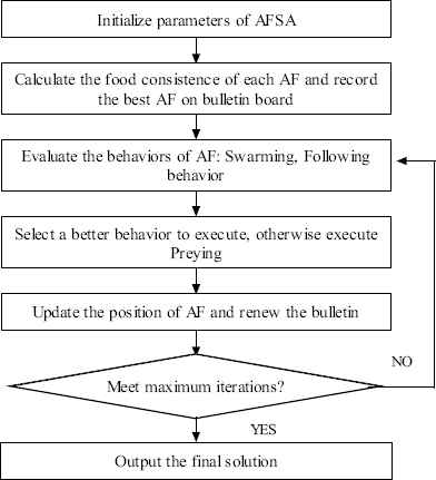
The framework of basic AFSA
3. Artificial Fish Swarm Algorithm with Estimation of Distribution (AFSA-ED)
The main components of the proposed AFSA-ED include the following strategies. Firstly, the pre-principle and the post-principle arranging mechanisms are applied to adjust the machine assignment and the operation sequence. Secondly, the preying behavior based on estimation of distribution is imitated by an object-oriented probability model. Thirdly, the attracting behavior is applied to improve the global search ability of algorithm. And finally, the local search based on critical path is applied to balance exploration and exploitation.
3.1. Pre-principle and post-principle Mechanisms
The FJSP optimizes the objective function by adjusting the machine assignment and the operation sequence. The order of solving the two sub-problems may affect the optimal results. Thus, we propose a pre-principle arranging mechanism and a post-principle arranging mechanism to adjust machine assignment and operation sequence. The objective is to enhance the diversity of population and make the algorithm searching the feasible solutions more comprehensively. The proposed mechanisms work as follows:
- (1)
Pre-principle arranging mechanism (PrA): The machine assignment part is firstly adjusted for balancing the workload of each machine, and then the operation sequence part is adjusted for minimizing the total makespan.
- (2)
Post-principle arranging mechanism (PoA): The operation sequence part is firstly adjusted for balancing the completion time of each job, and then the machine assignment part is adjusted for minimizing the total workload of machines.
While implementing the AFSA, the population is divided into two sub-populations. The two sub-populations respectively adopts the PrA and PoA mechanisms. After the independent evolution for each sub-populations, they are recombined to an entire population for further evolution.
3.2. The preying behavior based on estimation of distribution
In an AFSA system, preying behavior usually tends to be blindfold since the selection of destination locations is achieved by a random process. To overcome this shortcoming, we propose to estimate the distribution of the individuals, and then use the distribution model to guide preying behavior. The estimation of distribution algorithm (EDA) can reduce the randomness of behavior and make the search move toward and converge to the promising regions in the solution space.
The EDA works as follows: (1) Select a set of promising individuals from the population according to the fitness value; (2) Estimate the probability distribution of the selected individuals according to a probabilistic model. The probability distribution is constructed by two matrixes, i.e., the machine probabilistic matrix and the operation probabilistic matrix; (3) Generate new individuals according to the estimated probability.
Let I denote the number of promising individuals selected from the current population, and
Let
While implementing the preying behavior, a new individual is generated by sampling the two probabilistic matrixes. The machine assignment vector is generated through sampling the probabilistic matrix
3.3. Attracting behavior
In AFSA, each AF determines its next position according to current state and its environmental state within its visible region, which may limit the exploration ability and interaction with the other AFs outside its visible region. We propose an attracting behavior to enhance exploration ability.
The bulletin board that records the state of the current optimal individual is setup. For each AF, it reads the position information of the optimal individual from the bulletin board, and then it moves one step toward this direction.
Suppose Xi is the current position of AFi, Yi, is the fitness value. Xbest is the position of the global optimal individual and its fitness value is Ybest. If Yi > Ybest, then AFi, moves towards Xbest for a step according to Eq. (2). Otherwise, if Yi > Ybest, which means that it is the optimal individual, then it executes default preying behavior.
3.4. Critical Path Local Search based on Public Factor
In this subsection, a local search procedure is presented to enhance the exploitation around the best solution obtained by the AFSA. The local search is based on the critical path, so it is applied to the schedule represented by the disjunctive graph rather than by the AF. Hence, when a solution is to be improved by the local search, it should be firstly decoded to a schedule represented by the disjunctive graph.
3.4.1. The disjunctive graph
A feasible solution of FJSP can be represented by the disjunctive graph G = (N,B ∪ C), where N is a set of nodes which includes all the operations and two dummy nodes: starting and terminating; B is a set of conjunctive arcs which represents precedence constraints in the same job; C is a set of disjunctive arcs which correspond to the precedence of operations processed on the same machine. The weight of each node is the processing time of corresponding operation. In a disjunctive graph, the longest path form the starting node to terminating node is called critical path, whose length determines the makespan of the schedule. Any operation on the critical path is called critical operation.
Take the problem shown in Table 1 for instance, a possible schedule represented by the disjunctive graph is showed in Fig. 2. SG and EG are respectively dummy starting and terminating nodes. The operations O1,1 and O2,3 are performed on M1 successively, O2,1 and O1,2 are performed on M3 successively, and O2,2 is processed in M2.
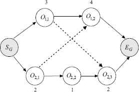
Illustration of framework of disjunctive graph
3.4.2. Neighborhood structure based on public factor
The disjunctive graph usually has more than one critical paths. Only changing the length of all the critical paths, the makespan can be changed. For obtaining a better schedule from the current one, lots of operations may be tried to move. The process is time consuming. So the public factor based critical path search in the neighborhoods is proposed. The public factor is used to identify the influence degree of the critical for all the critical paths. The public factor of an operation Oi,j can be defined by the formula:
While moving an operation, the precedence constrains should be satisfied. For an operation Oi,j processed on Mk, we define SEG(Oi,j) as the earliest start time and CEG(Oi,j) = SEG(Oi,j) + ti, j, k as the earliest completion time. Similarly, denote the latest start time without delaying the makespan as SLG(Oi,j) and the latest completion time as CLG(Oi,j) = SLG(Oi,j) + ti, j, k. Let PJi,j = Oi, j−1 be the precedent of operation Oi,j and FJi,j = Oi, j+1 be the successor of operation Oi,j. Denote PMi,j as the operation performed on Mk right before Oi,j and SMi,j as the operation performed on Mk right after Oi,j. In the disjunctive graph G, the process of moving an operation Oi,j is to delete it from its current machine sequence by moving all its disjunctive arcs and then insert it at another available machine by adding disjunctive arcs. Let POl (l = 1,2, ..., x) be the critical operation to be moved, where x is the total number of critical operations in G. Let G− be the disjunctive graph obtained by deleting the critical operation POl from G. For no increasing the makespan after inserting operation POl, we take Cmax(G) as the makespan of G− when we calculate the latest start time SLG− (Oi,j) for each operation in G−. If POl is inserted before Oi,j on machine Mk in G−, it could be started as early as CEG− (PMi,j) and should be completed as late as SLG− (Oi,j) without delaying the required makespan Cmax(G). In addition, POl needs to comply with the operation precedence constraints. So, the available idle time for inserting POl to machine Mk need to satisfy the following condition:
This moving process is repeated until a better schedule strategy is found or all critical operations have been tried to move. The procedure of local search is shown in Algorithm 1.
| 1. | Convert the feasible schedule to the disjunctive graph G |
| 2. | Get all the critical operations in the G |
| 3. | Calculate the Pf of all the critical operations and sort them in descending order to form a set {PO1, PO2,...POx} |
| 4. | for i = 1 to x do |
| Delete POi from G to get G− | |
| Calculate all the idle time intervals in G− | |
| if existing an available time interval for POi | |
| then | |
| Insert the operation POi to get Gi | |
| Return the disjunctive graph Gi | |
| end if | |
| end for | |
| 5. | Return the final disjunctive graph. |
The procedure of critical path local search
Figure 3 gives an illustration of the local search for the example in Table 1. In Fig. 3 (a), the only critical path is SG → O1,1 → O2,1 → O2,2 → O2,3→ EG, and the makespan is 17. The critical operation set is POl = {O1,1, O2,1, O2,2, O2,3}, and all the public factors for the critical operations are 1. So we can try to move the critical operations O1,1, O2,1, O2,2, and O2,3 successively. In this process, the algorithm preferentially selects the machine with the least processing time is and then judges the feasibility according to Eq. (6). Fig. 3 (b) show the disjunctive graph G1 obtained by moving the critical operation O1,1 to machine M1. In this case, the makespan is reduced to 12. Fig. 3 (c) show the disjunctive graph G2 obtained by moving the critical operation O2,1 to machine M3. IN this case, the makespan is 11. Following this, the critical operation O2,2 is not satisfied the moving condition according to Eq. (6). Finally, the algorithm obtains the disjunctive graph Fig. 3 (d) by moving the critical operation O2,3 to machine M4. In this case, the makespan is reduced to 9.
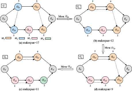
Illustration of the local search
4. The Implementation of AFSA-ED for FJSP
In this section, we will give the implementation of the AFSA-ED for FJSP. Firstly, the representation of the AF, decoding method and the population initialization are introduced. Then, the framework of the algorithm is presented.
4.1. Representation and movement
In AFSA-ED, each AF represents a feasible solution of the problem. Each AF is expressed by two vectors: machine assignment vector and operation sequence vector, which correspond to the two sub-problems of the FJSP. The machine assignment vector is represented by a vector of N integer values and N is the total number of operations. Each element of vector denotes the machine selection of each operation and the value is the index of the array of alternative machine set. The operation sequence vector is an un-partitioned permutation with repetitions of job Ji (i = 1,2,...,n). The length of operation sequence vector equals to N. The index i of job Ji occurs ni times in the vector, and the k-th occurrence of a job number refers to the k-th operation in the technological sequence of this job.
For the problem in Table 1, a representation of a feasible solution is shown in Fig. 4. The machine assignment vector is (1,2,2,2,3). If the operation O2,1 is processed on {M2, M3, M4}, then the corresponding element ‘2’ means that operation O2,1 will be assigned to the second machine M3. If the operation sequence is given as (2,1,2,2,1), then scanning the vector from left to right, the processing order of operations can be obtained: O2,1 − O1,1 − O2,2 − O2,3 − O1,2.
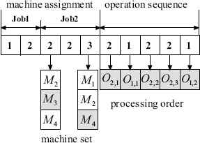
Illustration of the representation of a solution
To address the discrete FJSP, the movement of an AF in the solution space is completed by learning the partial structure from the target AF. Fig. 5 gives an illustrative example of the movement process. Assume the i-th AF is (1,2,2,2,3;2,1,2,2,1) in the current generation, and its target AF is (2,2,1,3,2;1,2,2,1,2), then an indicator vector with the same length is produced by randomly filled with the elements of the set {0, 1}. The number of the element “1” is
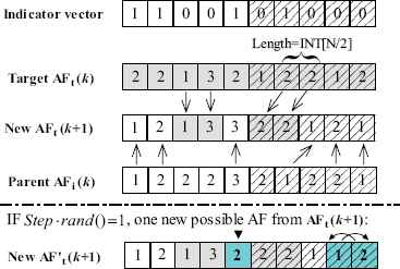
Illustration of the movement of an AF
4.2. Decoding of AF
For calculating the value of the makespan, each individual in the artificial fish swarm is decoded to the corresponding schedule sequence. The decoding is achieved by the process that assigns operations to the machines at their earliest possible starting time according to technological order of the jobs. It is worth noticing that the scheduling acquired in this way is semi-active. Then the active decoding is applied, which checks the possible blank time interval before appending an operation at the last position, and fills the first blank interval before the last operation to convert the semi-active schedule to an active one so that the makespan can be shorten34.
4.3. Initialization
In this subsection, an integrated initialization algorithm is proposed for machine assignment initialization and operation sequence initialization. To generate the initial machine assignments, the following rules are applied:
- (1)
Global approach of localization (GAL)17.
- (2)
Local approach of localization (LAL).
- (3)
Random rule.
The LAL makes a random permutation for the positions of machines. Following this, for each operation, it selects the machine with minimum processing time in the alternative machine set, and updates the machine workload by adding this processing to the processing time of the remaining unarranged operations within the same job. Take the problem showed in Table 1 as an example, Table 2 shows a possible machine assignment obtained by using the LAL. The last four columns indicate the final assignments obtained by LAL. In the table, the items in bold type are the updated workload of machines, and the “-” means that the operation cannot be processed on the corresponding machine.
| M3 | M2 | M4 | M1 | M3 | M2 | M4 | M1 | M3 | M2 | M4 | M1 | ... | M3 | M2 | M4 | M1 | |
|---|---|---|---|---|---|---|---|---|---|---|---|---|---|---|---|---|---|
| O1,1 | - | 5 | 6 | 3 | - | 5 | 6 |  |
- | 5 | 6 | |
… | - | 5 | 6 | |
| O1,2 | 4 | - | 5 | 6 | 4 | - | 5 | 9 |  |
- | 5 | 9 | … | |
- | 5 | 9 |
| O2,1 | 2 | 5 | 3 | - | 2 | 5 | 3 | - | 2 | 5 | 3 | - | … |  |
5 | 3 | - |
| O2,2 | 5 | 1 | 3 | 1 | 5 | 1 | 3 | 1 | 5 | 1 | 3 | 1 | 7 |  |
3 | 1 | |
| O2,3 | - | 3 | 2 | 2 | - | 3 | 2 | 2 | - | 3 | 2 | 2 | - | 4 | |
2 |
Initial assignments by LAL
The random rule executes by randomly selecting a machine from the alternative machine set for each operation. The GAL emphasizes the global workload among all the machines. The advantage of the LAL is that it obtains different initial assignments in different runs of the algorithm and emphasizes the workload among the set of machines within the same job. In addition, the random rule can increase the diversity of initial population. In our algorithm, the above three rules are used in a hybrid way. More specially, the initial machine assignments of 30% solutions in the population are generated by the GAL, 50% solutions by the LAL, and 20% solutions by random rule.
In our algorithm, the initial operation sequences are generated by the following three dispatching rules:
- (1)
Most time remaining (MTR). The job with the most remaining processing time will be arranged first.
- (2)
Most number of operations remaining rule (MOR). The job with the most remaining unprocessed operations has a high priority to be arranged.
- (3)
Random rule. Randomly generate the sequence of the operations. In particular, the above three rules are used in a hybrid way, then 20% of initial operation sequences are generated by random rule, 40% by the MTR, and 40% by the MOR.
4.4. The framework of AFSA-ED
The framework of AFSA-ED for solving FJSP is shown in Fig. 6. At the beginning of each generation, the entire population is randomly divided into two equal size sub-populations with one sub-population using machine based mechanism, and the other sub-population using operation based mechanism. Each AF evaluates by executing swarming, following, attracting behaviors. If the algorithm obtains a better solution using the three behaviors, it selects a better behavior to execute, otherwise, it executes the default improved preying behavior. When all individuals complete the searching process, the two sub-populations are combined into an entire population. Then the optimal individual of the population executes the critical path based on local search for further exploitation. If a new better individual is obtained, then the bulletin board is updated accordingly. The algorithm stops when the maximum iteration time is reached.
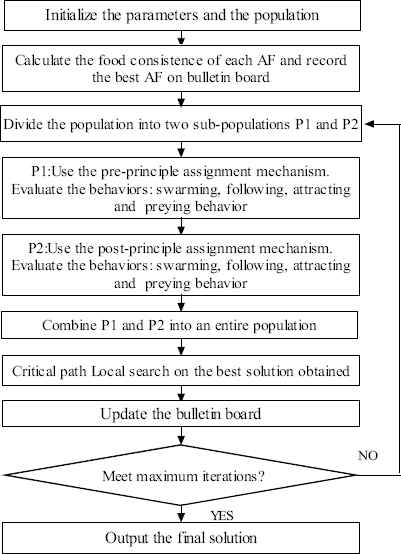
The framework of the AFSA-ED for the FJSP
5. Experimental Results
5.1. Instances and parameters
To evaluate the performance of the AFSA-ED, we consider three sets of well-known benchmarks with 160 instances:
- (1)
BRdata: The data set includes 10 instances from Brandimarte11. The number of jobs ranges from 10 to 20, the number of machines ranges from 4 to 15, and the flexibility of each operation ranges from 1.43 to 4.10.
- (2)
BCdata: The data set includes 21 instances from Barnes and Chambers35, which were acquired from the classical JSP mt10 and the la24, la40 instances. The number of jobs ranges from 10 to 15, the number of machines ranges from 11 to 18, and the flexibility of each operation ranges from 1.07 to 1.30.
- (3)
HUdata: The data set includes 129 instances from Hurink et al. 36, which were obtained from 3 classical JSP instances (mt06, mt10, mt20) by Fisher and Thompson and 40 classical JSP instances (la01–la40) by Lawrence. HUdata is divided into three subsets: Edata, Rdata, and Vdata. The number of jobs ranges from 6 to 30, the number of machines ranges from 5 to 15, and the flexibility of each operation ranges from 1.15 to 7.5.
The AFSA-ED is coded and implemented in matlab language on an Intel Core i5 2.53 GHz personal computer with 1GB of RAM. The algorithm runs 30 independent times for each instance from BRdata and BCdata, and runs 10 independent times for each instance from HUdata on account of the large number of instances in this data set. The computational results are compared with several performing algorithms from the existing literatures.
Each instance can be characterized by the following parameters: number of jobs (n), number of machines (m), number of operations (T0) and the flexibility of problem (Flex). The parameters in the AFSA-ED include population size (AFs), the maximum iteration times, the try number, the step of AF (Step), the visual of AF (Visual), and the crowd factor (delta). In our experiment, the iteration times and the try number are taken as 40. The settings of the other parameters for each data set are listed in Table 3.
| Data set | AFs | Step | Visual | delta |
|---|---|---|---|---|
| BRdata | 20 | 5 | 40 | 10 |
| BCdata | 40 | 10 | 100 | 20 |
| HUdata | 60 | 20 | 200 | 30 |
Parameter settings of the AFSA-ED
5.2. Computational results
The computational results for each data set are shown in this subsection. In the following tables, (LB,UB) denotes the lower and upper bounds37. The LB of BRdata and BCdata instances are taken from Mastrolilli12, while the LB of HUdata instances are computed by Jurisch.38 Cm denotes the best makespan. AV denotes the average makespan. SD denotes standard deviation of the makespan. Ta is the average running time of the algorithm in terms of seconds. To illustrate the quality of the results obtained by the AFSA and the compared algorithms, the mean relative error (MRE) is also introduced. The relative error (RE) is calculated as follows: RE = (MS − LB)/LB × 100%, where MS is the makespan obtained by the corresponding algorithm.
5.2.1. Influence of proposed EDA process
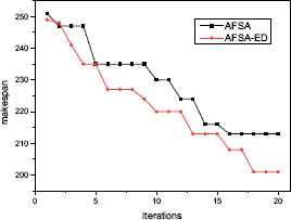
To investigate the influence of proposed EDA process for preying behavior, the experiments on the BRdata are conducted by implementing the AFSA-ED and the AFSA without EDA, respectively. The parameters in the AFSA are taken as the same in AFSA-ED, and the two algorithms runs 30 independent times for each instance. The results are given in Table 4. Compared with AFSA, AFSA-ED outperforms AFSA in all 10 instances for the average makespan and the best makespan, and the SD values obtained by AFSA-ED are relative smaller than AFSA for most of the instances. However, the overall computation time of the AFSA-ED is slightly longer than AFSA because of the EDA process. Fig. 7 and Fig. 8 show the convergence curves in solving MK7 and MK10 by AFSA-ED and AFSA respectively. The experiment results show the validity of the proposed EDA process for preying behavior.
| Instance | n × m | T0 | Flex. | (LB,UB) | ABC |
HHS |
AFSA |
AFSA-ED |
||||||||||
|---|---|---|---|---|---|---|---|---|---|---|---|---|---|---|---|---|---|---|
| Cm | AV | SD | Cm | AV | SD | Cm | AV | SD | Ta | Cm | AV | SD | Ta | |||||
| Mk01 | 10×6 | 55 | 2.09 | (36,42) | 40 | 40.00 | 0.00 | 40 | 40.00 | 0.00 | 40 | 41.25 | 0.65 | 1.39 | 40 | 40.00 | 0.00 | 2.59 |
| Mk02 | 10×6 | 58 | 4.01 | (24,32) | 26 | 26.50 | 0.50 | 26 | 26.63 | 0.49 | 28 | 29.04 | 0.58 | 1.61 | 26 | 26.10 | 0.30 | 2.82 |
| Mk03 | 15×8 | 150 | 3.01 | (204,211) | 204 | 204.00 | 0.00 | 204 | 204.00 | 0.00 | 204 | 204.00 | 0.00 | 1.00 | 204 | 204.00 | 0.00 | 1.12 |
| Mk04 | 15×8 | 90 | 1.91 | (48,81) | 60 | 61.22 | 1.36 | 60 | 60.03 | 1.18 | 64 | 65.51 | 1.03 | 5.68 | 60 | 60.27 | 0.72 | 12.94 |
| Mk05 | 15×4 | 106 | 1.71 | (168,186) | 172 | 172.98 | 0.14 | 172 | 172.80 | 0.41 | 177 | 177.69 | 0.47 | 4.75 | 172 | 172.40 | 0.48 | 10.49 |
| Mk06 | 10×15 | 150 | 3.27 | (33,86) | 60 | 64.48 | 1.75 | 58 | 59.13 | 0.63 | 62 | 63.86 | 0.72 | 20.58 | 57 | 58.60 | 0.75 | 39.27 |
| Mk07 | 20×5 | 100 | 2.83 | (133,157) | 139 | 141.42 | 1.20 | 139 | 139.57 | 0.50 | 142 | 143.03 | 0.95 | 28.47 | 139 | 140.63 | 0.71 | 57.63 |
| Mk08 | 20×10 | 225 | 1.43 | 523 | 523 | 523.00 | 0.00 | 523 | 523.00 | 0.00 | 523 | 523.00 | 0.00 | 1.04 | 523 | 523.00 | 0.00 | 2.14 |
| Mk09 | 20×10 | 240 | 2.53 | (299,369) | 307 | 308.76 | 1.63 | 307 | 307.00 | 0.00 | 310 | 310.75 | 0.54 | 4.06 | 307 | 307.13 | 0.43 | 9.40 |
| Mk10 | 20×15 | 240 | 2.98 | (165,296) | 208 | 212.84 | 2.43 | 205 | 211.13 | 2.37 | 213 | 214.91 | 1.37 | 50.44 | 201 | 201.93 | 1.06 | 104.10 |
Results of ten BRdata instances

Convergence curves of MK07
Convergence curves of MK10
5.2.2. Results of BRdata problems
The AFSA-ED is first tested on ten instances of BRdata. Meanwhile, we make a comparison with ABC algorithm by Wang et al.39 and HHS algorithm by Yuan et al.40. These results are also given in Table 4. It can be seen that AFSA-ED, ABC and HHS obtain the same best result for instances Mk01-Mk05, and Mk07-Mk09. For Mk06 and Mk10, AFSA-ED obtains the values of 57 and 201, respectively. On the other hand, the ABC obtains the best values of 60 and 208, respectively, and HHS obtains the best values of 58 and 205, respectively. Compared with ABC, AFSA-ED outperforms ABC in all 10 instances for the average makespan, and the SD values of AFSA-ED are relative smaller than ABC. In comparison with HHS, AFSA-ED outperforms HHS in 7 out 10 instances for the average makespan. It is worth noting that AFSA-ED can obtain average value of 201.93 and SD value of 1.06 for instance Mk10, respectively. On the other hand, the HHS can obtain average value of 211.13 and SD value of 2.37, respectively.
In addition, Table 5 gives a detailed comparison in terms of the MRE of the best value and the MRE of average value. We compare AFSA-ED with the PVNS of Yazdani et al.41, the CDDS of Ben Hmida et al.37, the BEDA of Wang et al.42, the ABC and the HHS. BKS represents the best known solution ever reported in the literature for each instance. It can be seen that AFSA-ED finds 9 best known solutions for 10 instances. The AFSA-ED obtains the MRE of the best value which is equal to 14.85%, while PVNS, CDDS, ABC, BDEA, and HHS are 16.43%, 14.98%, 16.19%, 16.07%, and 15.40%, respectively. For the MRE of average value obtained, AFSA-ED generates 15.64%, faced to 16.48% for HHS, 17.01% for PVNS, 18.55% for ABC, and 19.24 % for BDEA. However, faced to 15.34 % for the CDDS algorithm, the AFSA-ED Obtains a higher MRE. The Gantt chart of solution of MK06 obtained by AFSA-ED is showed in Fig. 9.
| Instance | BKS | AFSA-ED |
PVNS |
CDDS |
|||
|---|---|---|---|---|---|---|---|
| Cm(AV) | MRE | Cm(AV) | MRE | Cm(AV) | MRE | ||
| Mk01 | 40 | 40 (40) | 11.11(11.11) | 40 (40) | 11.11(11.11) | 40 (40) | 11.11(11.11) |
| Mk02 | 26 | 26(26.10) | 8.33(8.75) | 26(26.04) | 8.33(8.50) | 26(26) | 8.33(8.33) |
| Mk03 | 204 | 204(204) | 0.00(0.00) | 204(204) | 0.00(0.00) | 204(204) | 0.00(0.00) |
| Mk04 | 60 | 60(60.27) | 25.00(25.56) | 60(60.60) | 25.00(26.25) | 60(60) | 25.00(25.00) |
| Mk05 | 172 | 172(172.40) | 2.38(2.62) | 173(173) | 2.98(2.98) | 173(173.5) | 2.98(3.27) |
| Mk06 | 57 | 57(58.60) | 72.73(77.57) | 60(61) | 81.82(84.85) | 58(59) | 75.76(78.79) |
| Mk07 | 139 | 139(140.63) | 4.51(5.73) | 141(141.2) | 6.02(6.17) | 139(139) | 4.51(4.51) |
| Mk08 | 523 | 523(523) | 0.00(0.00) | 523(523) | 0.00(0.00) | 523(523) | 0.00(0.00) |
| Mk09 | 307 | 307(307.13) | 2.68(2.72) | 308(308.8) | 3.01(3.28) | 307(307) | 2.68(2.68) |
| Mk10 | 197 | 201(201.93) | 21.82(22.38) | 208(209.4) | 26.06(26.91) | 197(197.75) | 19.39(19.85) |
| MRE | 14.85(15.64) | 16.43(17.01) | 14.98(15.34) | ||||
| Instance | BKS | ABC |
BEDA |
HHS |
|||
|---|---|---|---|---|---|---|---|
| Cm(AV) | MRE | Cm(AV) | MRE | Cm(AV) | MRE | ||
| Mk01 | 40 | 40 (40) | 11.11(11.11) | 40 (41.02) | 11.11(13.94) | 40 (40) | 11.11(11.11) |
| Mk02 | 26 | 26(26.50) | 8.33(10.24) | 26(27.25) | 8.33(13.54) | 26(26.63) | 8.33(10.96) |
| Mk03 | 20 | 204(204) | 0.00(0.00) | 204(204) | 0.00(0.00) | 204(204) | 0.00(0.00) |
| Mk04 | 60 | 60(61.22) | 25.00(27.54) | 60(63.69) | 25.00(32.69) | 60(60.03) | 25.00(25.06) |
| Mk05 | 172 | 172(172.98) | 2.38(2.96) | 173(173.38) | 2.98(3.20) | 172(172.80) | 2.38(2.86) |
| Mk06 | 57 | 60(64.48) | 81.82(95.39) | 60(62.83) | 81.82(90.39) | 58(59.13) | 75.76(79.18) |
| Mk07 | 139 | 139(141.42) | 4.51(6.33) | 139(141.55) | 4.51(6.43) | 139(139.57) | 4.51(4.94) |
| Mk08 | 523 | 523(523) | 0.00(0.00) | 523(523) | 0.00(0.00) | 523(523) | 0.00(0.00) |
| Mk09 | 307 | 307(308.76) | 2.68(2.93) | 307(310.35) | 2.68(3.80) | 307(307) | 2.68(2.68) |
| Mk10 | 197 | 208(212.84) | 26.06(28.99) | 206(211.92) | 24.85(28.44) | 205(211.13) | 24.24(27.96) |
| MRE | 16.19(18.55) | 16.07(19.24) | 15.40(16.48) | ||||
Comparison between AFSA-ED and several existing algorithms on BRdata
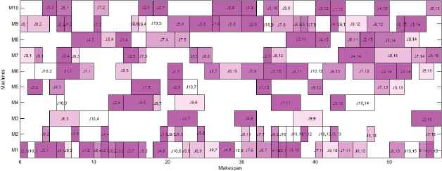
Gantt chart of solution of MK06 obtained by AFSA-ED (makespan = 57)
To determine the statistical differences between the AFSA-ED and the compared algorithms, the Friedman test and Holm procedure are conducted. The results are presented in Table 6. It can be seen from the Friedman test results that the differences among the six algorithms are statistically relevant with 98% certainty. The AFSA-ED obtains the best overall rank. The holm procedure shows that the AFSA-ED obtains better results than the compared five algorithms, and the differences are statistically relevant with 97%, 66%, 81%, 86%, and 67% certainty, respectively.
| Friedman test | Holm procedure | ||||||
|---|---|---|---|---|---|---|---|
| Algorithm | Rank | χ2 | 1 − p value | Diff.? | Algorithm | z | 1 − p value |
| AFSA-ED | 2.85 | 14.42 | 0.98 | Yes | - | - | - |
| PVNS | 4.50 | AFSA-ED v.s. PVNS | 1.97 | 0.98 | |||
| CDDS | 3.20 | AFSA-ED v.s. CDDS | 0.41 | 0.66 | |||
| ABC | 3.60 | AFSA-ED v.s. ABC | 0.89 | 0.81 | |||
| BEDA | 3.75 | AFSA-ED v.s. BEDA | 1.07 | 0.86 | |||
| HHS | 3.10 | AFSA-ED v.s. HHS | 0.29 | 0.67 | |||
Friedman test and Holm procedure of different algorithms
5.2.3. Results of BCdata problems
In this subsection, we carry out experiments on 21 instances of BCdata. The detail computational results are reported and compared with the CDDS and the HDE-N1 of Yuan et al.43 in Table 7. As can be seen from Table 7, AFSA-ED outperforms CDDS and HDE-N1 in 10 out of 21instances. For the cases of seti5xxx and seti5xyz, CDDS obtains the best results of three algorithms, while AFSA-ED obtains better results than HDE-N1. The average values and SD values of AFSA-ED are better than HDE-N1. AFSA-ED offers the comparable results with HDE-N2 while being faster than HDE-N2.
| Instance | n × m | Flex | (LB,UB) | CDDS | HDE-N1 | HDE-N2 | AFSA-ED | ||||||||||
|---|---|---|---|---|---|---|---|---|---|---|---|---|---|---|---|---|---|
| Cm | AV | Cm | AV | SD | Ta(s) | Cm | AV | SD | Ta(s) | Cm | AV | SD | Ta(s) | ||||
| mt10x | 10×11 | 1.10 | (655,929) | 918 | 918 | 918 | 922.86 | 6.11 | 21.43 | 918 | 918.58 | 2.20 | 179.22 | 918 | 918.00 | 0.00 | 23.47 |
| mt10xx | 10×12 | 1.20 | (655,929) | 918 | 918 | 918 | 922.04 | 6.31 | 21.70 | 918 | 918.38 | 1.90 | 179.84 | 918 | 918.53 | 1.35 | 20.91 |
| mt10xxx | 10×13 | 1.30 | (655,936) | 918 | 918 | 918 | 919.94 | 3.96 | 23.05 | 918 | 918.00 | 0.00 | 179.39 | 918 | 918.17 | 0.37 | 25.38 |
| mt10xy | 10×12 | 1.20 | (655,913) | 906 | 906 | 905 | 906.52 | 1.09 | 22.51 | 905 | 905.56 | 0.79 | 169.77 | 905 | 905.23 | 0.55 | 22.80 |
| mt10xyz | 10×13 | 1.30 | (655,849) | 849 | 850.5 | 847 | 856.80 | 3.99 | 21.79 | 847 | 851.14 | 4.65 | 160.24 | 847 | 851.07 | 2.93 | 24.63 |
| mt10c1 | 10×11 | 1.10 | (655,927) | 928 | 928.5 | 927 | 928.92 | 1.96 | 21.07 | 927 | 927.72 | 0.45 | 174.19 | 927 | 927.20 | 0.47 | 23.35 |
| mt10cc | 10×12 | 1.20 | (655,914) | 910 | 910.75 | 910 | 913.92 | 3.40 | 21.00 | 908 | 910.60 | 2.40 | 165.61 | 908 | 908.40 | 1.13 | 40.86 |
| setb4x | 15×11 | 1.10 | (846,937) | 925 | 925 | 925 | 931.50 | 2.48 | 33.04 | 925 | 925.82 | 2.11 | 338.30 | 925 | 925.83 | 1.79 | 35.89 |
| setb4xx | 15×12 | 1.20 | (847,930) | 925 | 925 | 925 | 930.38 | 3.29 | 29.76 | 925 | 925.64 | 1.98 | 336.24 | 925 | 925.56 | 1.72 | 38.64 |
| setb4xxx | 15×13 | 1.30 | (846,925) | 925 | 925 | 925 | 931.42 | 3.59 | 29.89 | 925 | 925.48 | 1.68 | 353.55 | 925 | 925.60 | 1.45 | 36.42 |
| setb4xy | 15×12 | 1.20 | (845,924) | 916 | 916 | 910 | 921.38 | 4.44 | 31.13 | 910 | 914.00 | 3.50 | 330.18 | 910 | 913.90 | 2.70 | 36.50 |
| setb4xyz | 15×13 | 1.30 | (838,914) | 905 | 906.5 | 905 | 913.40 | 4.21 | 30.39 | 903 | 905.28 | 1.16 | 314.64 | 903 | 904.06 | 0.85 | 76.28 |
| setb4c9 | 15×11 | 1.10 | (857,924) | 919 | 919 | 914 | 919.32 | 2.87 | 32.19 | 914 | 917.12 | 2.52 | 313.02 | 914 | 916.26 | 2.17 | 64.27 |
| setb4cc | 15×12 | 1.20 | (857,909) | 909 | 910.5 | 909 | 912.58 | 3.81 | 32.00 | 907 | 909.58 | 1.89 | 316.89 | 907 | 908.00 | 1.13 | 83.61 |
| seti5x | 15×16 | 1.07 | (955,1218) | 1201 | 1201.5 | 1204 | 1215.48 | 5.36 | 73.20 | 1200 | 1205.64 | 3.43 | 1112.77 | 1198 | 1202.95 | 2.64 | 153.82 |
| seti5xx | 15×17 | 1.13 | (955,1204) | 1199 | 1199 | 1202 | 1205.66 | 2.56 | 72.52 | 1197 | 1202.68 | 2.02 | 1078.60 | 1198 | 1201.23 | 1.99 | 93.12 |
| seti5xxx | 15×18 | 1.20 | (955,1213) | 1197 | 1197.5 | 1202 | 1206.10 | 3.18 | 72.07 | 1197 | 1202.26 | 2.37 | 1087.12 | 1197 | 1202.63 | 2.24 | 97.86 |
| seti5xy | 15×17 | 1.13 | (955,1148) | 1136 | 1138 | 1138 | 1146.86 | 5.04 | 78.98 | 1136 | 1137.98 | 2.82 | 1250.62 | 1136 | 1138.13 | 1.98 | 142.65 |
| seti5xyz | 15×18 | 1.20 | (955,1127) | 1125 | 1125.3 | 1130 | 1137.44 | 3.42 | 80.85 | 1125 | 1129.76 | 2.44 | 1244.22 | 1125 | 1129.53 | 1.76 | 405.74 |
| seti5c12 | 15×16 | 1.07 | (1027,1185) | 1174 | 1174.5 | 1175 | 1182.54 | 7.62 | 69.06 | 1171 | 1175.42 | 1.63 | 1141.43 | 1174 | 1174.67 | 1.02 | 313.40 |
| seti5cc | 15×17 | 1.13 | (955,1136) | 1136 | 1137 | 1137 | 1145.62 | 5.58 | 78.83 | 1136 | 1137.76 | 2.48 | 1222.53 | 1136 | 1137.73 | 1.60 | 324.07 |
Comparison of AFSA-ED with CDDS and HDE-N1 on BCdata
Table 8 lists the best makespan and the MRE of AFSA-ED, TSBM2h by Bozejko et al. 13, CDDS37, IFS by Oddi et al. 44, HDE-N1 and HDE-N2 by Yuan et al.43. For the IFS algorithm, its performance depends on the relaxing factor γ, the table lists the results obtained by running IFS with γ ranging from 0.2 to 0.7, respectively. The difference between HDE-N1 and HDE-N2 is neighborhood structure. Moreover, HDE-N2 is more effective than HDE-N1, but its computational time is much longer than HDE-N1. From Table 8, as for the best makespan obtained, AFSA-ED obtains 85% of best known solutions, while TSBM2h obtains 81%, CDDS obtains 52%, IFS obtains 47%, HDE-N1 obtains 52%, and HDE-N2 obtains 95%. It can be seen that HDE-N2 outperforms AFSA-ED on two instances (seti5xxx, seti5c12), while AFSA-ED outperforms HDE-N2 on one instance (seti5x). In particular, the MRE of best makespan of AFSA is 22.39%, faced to 22.45% for TSBM2h, 22.54% for CDDS, 22.55% for HDE-N1, 23.09% for IFS (γ = 0.7), and 22.39% for HDE-N2. We note that AFSA-ED performs better than the TSBM2h, CDDS, IFS and HDE-N1, while the same with HDE-N2. However, the HDE-N2 tends to spend long time for finding best solutions. To determine the statistical differences among the AFSA-ED and the compared algorithms, the Friedman test and Holm procedure are also conducted. The results are presented in Table 9. It can be seen that the differences among the six algorithms are statistically relevant with 100% certainty. The AFSA-ED and the HDE-N2 obtain the best overall rank. The Holm procedure shows that the AFSA-ED obtains the same results with the HDE-N2. The Holm procedure also shows that the AFSA-ED obtains better results than other four algorithms, and the differences are statistically relevant with 62%, 94%, 100%, and 94%, respectively.
| Instance | BKS | AFSA-ED | TSBM2h | CDDS | IFS |
HDE-N1 | HDE-N2 | |||||
|---|---|---|---|---|---|---|---|---|---|---|---|---|
| 0.2 | 0.3 | 0.4 | 0.5 | 0.6 | 0.7 | |||||||
| mt10x | 918 | 918 | 922 | 918 | 980 | 936 | 936 | 934 | 918 | 918 | 918 | 918 |
| mt10xx | 918 | 918 | 918 | 918 | 936 | 929 | 936 | 933 | 918 | 926 | 918 | 918 |
| mt10xxx | 918 | 918 | 918 | 918 | 936 | 929 | 936 | 926 | 926 | 926 | 918 | 918 |
| mt10xy | 905 | 905 | 905 | 906 | 922 | 923 | 923 | 915 | 905 | 909 | 905 | 905 |
| mt10xyz | 847 | 847 | 849 | 849 | 878 | 858 | 851 | 862 | 847 | 851 | 847 | 847 |
| mt10c1 | 927 | 927 | 927 | 928 | 943 | 937 | 986 | 934 | 934 | 927 | 927 | 927 |
| mt10cc | 908 | 908 | 908 | 910 | 926 | 923 | 919 | 919 | 910 | 911 | 910 | 908 |
| setb4x | 925 | 925 | 925 | 925 | 967 | 945 | 930 | 925 | 937 | 937 | 925 | 925 |
| setb4xx | 925 | 925 | 925 | 925 | 966 | 931 | 933 | 925 | 937 | 929 | 925 | 925 |
| setb4xxx | 925 | 925 | 925 | 925 | 941 | 930 | 950 | 950 | 942 | 935 | 925 | 925 |
| setb4xy | 910 | 910 | 910 | 916 | 910 | 941 | 936 | 936 | 916 | 914 | 910 | 910 |
| setb4xyz | 903 | 903 | 903 | 905 | 928 | 909 | 905 | 905 | 905 | 905 | 905 | 903 |
| setb4c9 | 914 | 914 | 914 | 919 | 926 | 937 | 926 | 926 | 920 | 920 | 914 | 914 |
| setb4cc | 907 | 907 | 907 | 909 | 929 | 917 | 907 | 914 | 907 | 909 | 909 | 907 |
| seti5x | 1198 | 1198 | 1198 | 1201 | 1210 | 1199 | 1199 | 1205 | 1207 | 1209 | 1204 | 1200 |
| seti5xx | 1197 | 1198 | 1197 | 1199 | 1216 | 1199 | 1205 | 1211 | 1207 | 1206 | 1202 | 1197 |
| seti5xxx | 1197 | 1197 | 1197 | 1197 | 1205 | 1206 | 1206 | 1199 | 1206 | 1206 | 1202 | 1197 |
| seti5xy | 1136 | 1136 | 1136 | 1136 | 1175 | 1171 | 1175 | 1166 | 1156 | 1148 | 1138 | 1136 |
| seti5xyz | 1125 | 1125 | 1128 | 1125 | 1165 | 1149 | 1130 | 1134 | 1144 | 1131 | 1130 | 1125 |
| seti5c12 | 1171 | 1174 | 1174 | 1174 | 1196 | 1209 | 1200 | 1198 | 1198 | 1175 | 1175 | 1171 |
| seti5cc | 1136 | 1136 | 1136 | 1136 | 1177 | 1155 | 1162 | 1166 | 1138 | 1150 | 1137 | 1136 |
| MRE | 22.39 | 22.45 | 22.54 | 25.48 | 24.25 | 24.44 | 23.96 | 23.28 | 23.09 | 22.55 | 22.39 | |
Comparison of results using different algorithms (AFSA-ED, TSBM2h, CDDS, IFS, HDE)
| Friedman test | Holm procedure | ||||||
|---|---|---|---|---|---|---|---|
| Algorithm | Rank | χ2 | 1-p value | Diff.? | Algorithm | z | 1-p value |
| AFSA-ED | 2.76 | 143.05 | 1.00 | Yes | - | - | - |
| TSBM2h | 3.10 | AFSA-ED v.s. TSBM2h | 0.33 | 0.62 | |||
| CDDS | 4.36 | AFSA-ED v.s. CDDS | 1.56 | 0.94 | |||
| IFS 0.2 | 9.79 | AFSA-ED v.s. IFS 0.2 | 6.86 | 1.00 | |||
| IFS 0.3 | 8.88 | AFSA-ED v.s. IFS 0.3 | 5.97 | 1.00 | |||
| IFS 0.4 | 8.45 | AFSA-ED v.s. IFS 0.4 | 5.55 | 1.00 | |||
| IFS 0.5 | 7.95 | AFSA-ED v.s. IFS 0.5 | 5.07 | 1.00 | |||
| IFS 0.6 | 6.71 | AFSA-ED v.s. IFS 0.6 | 3.85 | 1.00 | |||
| IFS 0.7 | 6.83 | AFSA-ED v.s. IFS 0.7 | 3.97 | 1.00 | |||
| HDE-N1 | 4.40 | AFSA-ED v.s. HDE- N1 | 1.60 | 0.94 | |||
| HDE-N2 | 2.76 | AFSA-ED v.s. HDE- N2 | 0.00 | 0.50 | |||
Friedman test and Holm procedure of different algorithms on BC data
5.2.4. Results of HUdata problems
This subsection shows the results of AFSA-ED for HUdata benchmark instances. Table 10 presents the MRE of the best makespan and average makespan obtained by AFSA-ED, CDDS and HDE-N1. It can be seen that AFSA can obtain the MRE of best value of 2.30%, 1.24% and 0.20% for Edata, Rdata and Vdata, respectively, while CDDS can obtain the MRE of best value of 2.32%, 1.34% and 0.12%, respectively, HED-N1 can obtain the MRE of best value of 2.35%, 1.28% and 0.26%, respectively. Compared with CDDS, AFSA-ED could obtain better results than CDDS for some instances of Edata (la16-la35), some instances of Rdata (la01-la15, la31-la40), and some instances of Vdata (la01-la05, la26-la30). For the MRE of best and average makespan, AFSA-ED outperforms CDDS for Edata and Rdata, while CDDS obtains the best result of three algorithms for Vdata. In comparison with HDE-N1, AFSA-ED can obtain better results than HDE for some instances of Edata (mt06/10/20, la21-35), some instances of Rdata (la01-10,la21-40) and some instances of Rdata (la06-10,la21-35). For the MRE of best and average makespan, AFSA-ED outperforms HDE-N1 for three datasets.
| Instance | n × m | Edata (Flex = 1.15) |
Rdata (Flex = 2.0) |
Vdata (Flex ∈ [2.5,7.5]) |
||||||
|---|---|---|---|---|---|---|---|---|---|---|
| CDDS | HDE-N1 | AFSA-ED | CDDS | HDE-N1 | AFSA-ED | CDDS | HDE-N1 | AFSA-ED | ||
| mt06/10/20 | 6×6 10×10 20×5 |
0.00 (0.05) | 0.05 (0.13) | 0.00 (0.08) | 0.34 (0.47) | 0.34 (0.45) | 0.34 (0.39) | 0.00 (0.00) | 0.00 (0.01) | 0.00 (0.00) |
| la01-la05 | 10×5 | 0.00 (0.73) | 0.00 (0.00) | 0.00 (0.00) | 0.11 (0.28) | 0.11 (0.31) | 0.08(0.22) | 0.13 (0.23) | 0.04 (0.19) | 0.09 (0.20) |
| la06-la10 | 15×5 | 0.00 (0.19) | 0.00 (0.10) | 0.00 (0.06) | 0.03 (0.19) | 0.05 (0.10) | 0.02 (0.15) | 0.00 (0.00) | 0.03 (0.10) | 0.07 (0.11) |
| la11-la15 | 20×5 | 0.29 (1.12) | 0.29 (0.29) | 0.29 (0.29) | 0.02 (0.37) | 0.00 (0.02) | 0.00 (0.22) | 0.00 (0.00) | 0.00 (0.01) | 0.00 (0.00) |
| la16-la20 | 10×10 | 0.49 (1.15) | 0.02 (0.48) | 0.04 (0.45) | 1.64 (1.90) | 1.64 (1.69) | 1.64 (1.65) | 0.00 (0.00) | 0.00 (0.00) | 0.00 (0.00) |
| la21-la25 | 15×10 | 5.70 (6.27) | 5.82 (6.41) | 5.66 (6.35) | 3.82 (4.26) | 3.73 (4.57) | 3.68 (4.46) | 0.70 (1.01) | 1.63 (2.15) | 1.40 (1.89) |
| la26-la30 | 20×10 | 3.96 (4.84) | 3.89 (4.71) | 3.78 (4.69) | 0.66 (0.98) | 1.04 (1.41) | 0.97 (0.84) | 0.11 (0.19) | 0.42 (0.63) | 0.09 (0.17) |
| la31-la35 | 30×10 | 0.42 (0.83) | 0.50 (0.59) | 0.37 (0.55) | 0.22 (0.41) | 0.22 (0.33) | 0.18 (0.33) | 0.02 (0.04) | 0.12 (0.18) | 0.07 (0.12) |
| la36-la40 | 15×15 | 9.10 (9.88) | 9.63 (10.43) | 9.64 (9.95) | 4.85 (4.97) | 3.98 (4.92) | 3.89 (4.88) | 0.00 (0.00) | 0.00 (0.01) | 0.00 (0.00) |
| MRE (%) | 2.32 (2.91) | 2.35 (2.68) | 2.30 (2.60) | 1.34 (1.59) | 1.28 (1.59) | 1.24 (1.51) | 0.12 (0.16) | 0.26 (0.38) | 0.20 (0.29) | |
Comparison of MRE obtained by using AFSA-ED, CDDS and HDE-N1 on HUdata
5.3. Discussions
In Table 11, we summarize the MRE of the best makespan obtained by our algorithm and other known algorithm for BRdata set, BCdata set and HUdata set. The first column shows the name of data set, the second column shows the number of problems for each set, the following nine columns show the MRE of AFSA-ED, GA of Chen15, TS of Mastrolilli 12, GA of Pezzella17, CDDS, PVNS, HHS, HDE-N1 and HDE-N2. As can be seen in Table 11, HDE-N2 achieves the state-of-the-art performance on three data sets. Except for HDE-N2, AFSA-ED outperforms the other seven algorithms on BRdata and BCdata; it outperforms GA_Chen, GA_Pezzella, PVNS and HHS on three sub-data sets of HUdata, and CDDS on Edata and Rdata. TS works better than AFSA-ED on the HUdata, and CDDS works better than AFSA-ED on Vdata. In particular, HDE-N2 is a time consuming algorithm, in which the computational time is about 5 times longer than AFSA-ED as shown in Table 7. In conclusion, the results show that the AFSA-ED is an effective algorithm for FJSP.
| Dada set | PNum | AFSA-ED | GA_Chen | TS | GA_Pezzella | CDDS | PVNS | HHS | HDE-N1 | HDE-N2 |
|---|---|---|---|---|---|---|---|---|---|---|
| BRdata | 10 | 14.85 | 19.55 | 19.55 | 17.53 | 14.98 | 16.39 | 15.40 | 15.58 | 14.67 |
| BCdata | 21 | 22.39 | 38.64 | 38.64 | 29.56 | 22.54 | 26.66 | 22.89 | 22.55 | 22.39 |
| Hurink Edata | 43 | 2.30 | 5.59 | 2.17 | 6.00 | 2.32 | 3.86 | 2.67 | 2.35 | 2.11 |
| Hurink Rdata | 43 | 1.24 | 4.41 | 1.24 | 4.42 | 1.34 | 1.88 | 1.88 | 1.28 | 1.05 |
| Hurink Vdata | 43 | 0. 20 | 2.59 | 0.095 | 2.04 | 0.12 | 0.42 | 0.39 | 0.26 | 0.080 |
MRE of the best makespan obtained by AFSA-ED and other known algorithms
6. Conclusion
In this paper, an efficient artificial fish swarm algorithm with estimation of distribution was proposed for solving the flexible job-shop scheduling problem with the criterion to minimize the makespan. Considering the interaction of two sub-problems, we propose the pre-principle and post-principle arranging mechanism to adjust machine assignment and operation sequence with different orders. For improving the global exploration of algorithm, we modify preying behavior with estimation of distribution and embed attracting behavior to the algorithm. To balance the exploration and exploitation, the critical path based local search was used. The proposed algorithm is tested on 160 well known benchmark instances and 121 best known solutions are found. The computational results and comparisons demonstrate that the proposed AFSA-ED outperforms several existing algorithms and is especially effective for the FJSP. In the future research, the AFSA could be used in multi-objective FJSP or many real world manufacturing systems.
Acknowledgements
The authors would like to thank the support of the National Natural Science Foundation of China (61572104, 61103146, 61402076, 61502072), Startup Fund for the Doctoral Program of Liaoning Province (20141023), the Fundamental Research Funds for the Central Universities (DUT15QY26, DUT15RC(3)088), and the project of the Key Laboratory of Symbolic Computation and Knowledge Engineering in Jilin University (93K172016K11).
References
Cite this article
TY  - JOUR
AU  - Hongwei Ge
AU  - Liang Sun
AU  - Xin Chen
AU  - Yanchun Liang
PY  - 2016
DA  - 2016/09/01
TI  - An Efficient Artificial Fish Swarm Model with Estimation of Distribution for Flexible Job Shop Scheduling
JO  - International Journal of Computational Intelligence Systems
SP  - 917
EP  - 931
VL  - 9
IS  - 5
SN  - 1875-6883
UR  - https://doi.org/10.1080/18756891.2016.1237190
DO  - 10.1080/18756891.2016.1237190
ID  - Ge2016
ER  -