
Manifold Regularized Proximal Support Vector Machine via Generalized Eigenvalue
- DOI
- 10.1080/18756891.2016.1256570How to use a DOI?
- Keywords
- Support vector machines; Generalized eigenvalues; Locality preserving projections; Manifold regularization
- Abstract
Proximal support vector machine via generalized eigenvalue (GEPSVM) is a recently proposed binary classification technique which aims to seek two nonparallel planes so that each one is closest to one of the two datasets while furthest away from the other. In this paper, we proposed a novel method called Manifold Regularized Proximal Support Vector Machine via Generalized Eigenvalue (MRGEPSVM), which incorporates local geometry information within each class into GEPSVM by regularization technique. Each plane is required to fit each dataset as close as possible and preserve the intrinsic geometric structure of each class via manifold regularization. MRGEPSVM is also extended to the nonlinear case by kernel trick. The effectiveness of the method is demonstrated by tests on some examples as well as on a number of public data sets. These examples show the advantages of the proposed approach in both computation speed and test set correctness.
- Copyright
- © 2016. the authors. Co-published by Atlantis Press and Taylor & Francis
- Open Access
- This is an open access article under the CC BY-NC license (http://creativecommons.org/licences/by-nc/4.0/).
1. Introduction
Standard SVMs1, which are powerful tools for data classification and regression, have come to play a very dominant role in machine learning and pattern recognition community. The approach is systematic and motivated by Statistical Learning Theory2, which seeks the optimal separating hyperplane by minimizing structural risk instead of empirical risk. In binary classification, it assigns the point to one of the two disjoint half spaces in either the original input space or a higher dimensional feature space. In order to find the optimal separating hyperplane, SVMs need to solve a quadratic programming problem (QPP) which is time-consuming in large sized samples.
Recently, several simpler classification methods were proposed3,4. Opposite to SVMs, in binary classification, they all aim at finding two planes so that each plane was closest to the points of its own class and furthest away from the points of the other class. This idea not only leads to faster and simpler algorithms than the conventional SVMs but also avoids the unbalanced sample distribution problem in SVMs. Among these methods, generalized eigenvalue proximal SVM (GEPSVM)5,6,7 does binary classification by formulating two eigenvalue problems instead of quadratic programming problem to generate two nonparallel planes which make it extremely fast in real-world applications. The eigenvectors corresponding to the smallest eigenvalues determines the above two planes, as shown in Fig. 1.
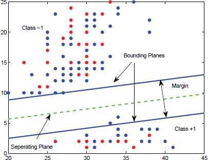
The examples of standard SVM
The last decade has witnessed the emergence of manifold learning as a vigorous paradigm for dimensionality reduction and data visualization. The basic assumption of manifold learning is that though probably each data point consists thousands of features, it may actually be sampled from a low dimensional manifold embedded in a high dimensional space. The popular manifold learning methods, including Locally Linear Embedding (LLE)8, ISOMAP9, Laplacian Eigenmap10 and their various extensions11,12, have gained successful applications in many fields. In addition to the applications in dimensionality reductions, manifold regularization13 has been proposed as a new form of regularization that allows us to exploit the geometry of the distribution of the data points. It has also been used in SVMs, e.g., Laplacian SVMs14,15, to take advantage of unlabeled data points. In the literature, manifold learning, especially locality preserving projections criteria16, are widely used to reduce dimensionality of the original data in feature extraction or penalize classifier using unlabeled data samples in semi-supervised learning. However, there is little evidence which has shown whether supervised classifier can benefit from manifold structure directly from labeled samples. Recently, the idea of manifold learning has been applied in GEPSVM by considering the local information within each class to eliminate the influence of outliers17.
With the geometric intuition of GEPSVM and the essence of manifold learning, we argue that manifold regularization is particularly suitable for GEPSVM and its variants. In contrast with conventional SVMs, GEPSVM and other recently proposed classifiers, e.g., Twin SVMs4,18, are all based on seeking planes best fitting the data points of the same class rather than just separating points of different classes. Twin SVMs are non-parallel planar classifiers whose target is to construct a classification hyper plane for two kinds of data, which makes the sample of each super plane distance as close as possible, and the distance of the samples as far as possible. In other words, they are not only “discriminative” based approach but also “expressive” based approach. Therefore, it’s natural to make attempts to combine manifold structure with these methods. Another reason is that the numerators of the objective functions of GEPSVM have similar formulations as least square regression which is known to tend to overfit data points. That’s why Tikhonov regularization terms19 are integrated in GEPSVM to enhance its generalization ability and avoid overfitting. But they merely penalize the numerators whereas ignoring the denominators. Furthermore, in many cases, manifold regularization is more powerful as it takes the intrinsic geometry structure of the data points into account. In this paper, manifold regularization, specifically locality preserving projections (LPP)20,21, is firstly extended in our context and then incorporated into classical GEPSVMs. Locality Preserving Projections (LPP) are linear projective maps that arise by solving a variation problem that optimally preserves the neighborhood structure of the data set22,23. LPP should be seen as an alternative to Principal Component Analysis (PCA)—a classical linear technique that projects the data along the directions of maximal variance. When the high dimensional data lies on a low dimensional manifold embedded in the ambient space, the Locality Preserving Projections are obtained by finding the optimal linear approximations to the Eigen functions of the Laplace Beltrami operator on the manifold24,25. LPP shares many of the data representation properties of nonlinear techniques such as Laplacian Eigen maps or Locally Linear Embedding. Yet LPP is linear and more crucially is defined everywhere in ambient space rather than just on the training data points. LPP may be conducted in the original space or in the reproducing kernel Hilbert space into which data points are mapped. This gives rise to kernel LPP. We should emphasize that the purpose of manifold regularization in our context is different from the classical one whose primary aim is to utilize the distribution information of unlabeled samples. Unlike semi-supervised26 learning, the intention of the proposed approach is to demonstrate how manifold structure of labeled samples is also beneficial to supervised learning even when unlabeled samples are available. Twin SVM is a non-parallel planar classifier shown in Fig. 2, its target is to construct a classification hyper plane for two kinds of data, which makes the sample of each super plane distance as close as possible, and the distance of the samples as far as possible.
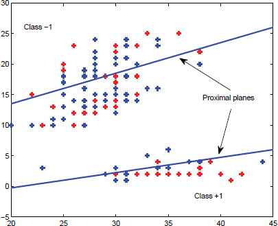
The examples of Twin SVM
In this paper, MRGEPSVM is derived by designing a modified locality preserving projections criteria and incorporating it into GEPSVM. Unlike conventional LPP, we project the data points onto planes and require the local geometry structure to be preserved. It demonstrates that manifold regularization is suitable for GEPSVM and its variants.
The remainder of this paper is organized as follows: In section 2, we give a brief overview of GEPSVM followed by the construction of local preserving projections criteria in section 3. Section 4 presents manifold regularized GEPSVM based on the novel regularization. In section 5, detailed experimental results are given and we conclude this paper in section 6.
2. A brief review of GEPSVM
Supposed we are given m1 training samples belongs to class 1 and m2 training samples belongs to class 2 in the n-dimensional real space, with m1 + m2 = m. Let A and B be two matrices whose rows are samples of class 1 and class 2 respectively. Let w1 and w2 be the normal to the two planes respectively, GEPSVM seeks two nonparallel planes given by:
3. Local Preserving Projections on Plane
In this section, the idea of local preserving projections is extended in the case that we expect the intrinsic geometry structure of original data samples of the same class can be preserved after they are projected to a plane.
Firstly, in order to preserve the original local geometry structure within each class, we need to construct a graph for each class, named as with-in class graph G(c)(c = 1,2). Each vertex in G(c) correspinds to a sample point which belongs to class c and an edge between a vertex pair is added when the corresponding sample pair is each other’s k-nearest neighbors. After the structure of G(c) is fixed, we need to determine its weight matrix S(c). In the literature, there exist several methods for weight calculation, e.g., RBF kernel, inverse Euclidean distance. In our experiments, RBF kernel is selected as follows:
After with-in graphs have been constructed in input space, we project the points of each class onto their corresponding fitting planes and extend LPP criteria under this condition. The detailed procedure is given as follows.
Give an arbitrary point x in ℝn and let y be its orthogonal projection onto the fitting plane wT x + b = 0, we can obtain the following equality from Fig. 3.
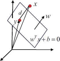
Illustration of the geometry of projecting x onto wT x + b = 0.
After a simple calculation as described in Ref. 15, the value of d can be expressed as:
On substituting (7) into (6), the orthogonal projection of x can be formulated as:
According to our idea, the local geometry structure within the points of each class should be preserved after the projection. Take class 1 for example, this leads to the following optimization problem.
By dropping the terms irrelative to optimize variables and making use of the expression of w1 and
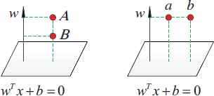
Illustration of the difference between LPP and the proposed projections
It’s obvious that the best vector that preserves local structure of data points corresponds to the worst plane doing so. As Fig. 4 left shows, A, B are projected meanwhile best preserving the local structure. However, in Fig. 4 right, a and b are projected, but they do not preserve the local structure.
4. Incorporate local geometry structure into GEPSVM
We are now in a position to introduce the new criteria (18) into classical GEPSVM. As aforementioned, GEPSVM aims to find two distinct planes which are not parallel to each other so that each closest to the points of one class and furthest away from the other. Recalling the objective function (5) of GEPSVM, it’s obvious that its numerator is similar to least square regression, which tends to generate overfitting solutions and that’s why we need regularization technique to avoid it. In original GEPSVM, Tikhonov regularization plays the role in tackling this problem. In this paper, besides Tikhonov term, manifold regularization, i.e., criteria (19), is also used to handle it.
Our idea is to seek two planes so that each one is required not only closest to the data set of its own and furthest from the other data set but also to preserve the local geometry structure of them, respectively. To achieve this, (10) is used to penalize the original GEPSVM, leading to the following modified objective functions for class 1.
Making the result of (19), (21) can be expressed as following:
We can view the second function as manifold regularized and incorporated into the first function as in (23) . At the same time, in order to balance the effect of the two objectives, trade-off factor δM is introduced, which leads to the following optimization problems.
Following the similar procedure above, we define an analogous minimization problem to (25) for determining Z2 = [w2; b2], i.e., the coefficient of the second plane
The minimum of (27) is achieved at the eigenvector corresponding to the smallest eigenvalue of the following generalized eigenvalue problem.
Once we obtain the eigenvectors corresponding to the smallest eigenvalues of (26) and (28), the two planes are determined at the same time. Therefore, for a new coming sample x, we first calculate the distance from x to the two planes given by (29):
Then we classify x as belonging to class 1 if otherwise d1 < d2 to class 2.
We now describe our simple algorithm as follows for implementing a linear MRGEPSVM.
Given m1 samples in ℝn represented by A ∈ ℝm1×n and m2 samples represented by B ∈ ℝm2×n:
|
Linear Manifold Regularized Proximal Support Vector Machine via Generalized Eigen-value
Originally, GEPSVM were proposed to tackle XOR problems which is difficult for conventional linear classifications such as SVMs, by which it can obtain nearly 100% correct. A “cross planes” example is show in Fig. 5 for GEPSVM and the proposed MRGEPSVM. We observe that MRGEPSVM obtains nearly the same accuracy as GEPSVM, which implies the ability of GEPSVM to solve XOR problems is not depressed in MRGEPSVM by introducing manifold regularization technique.
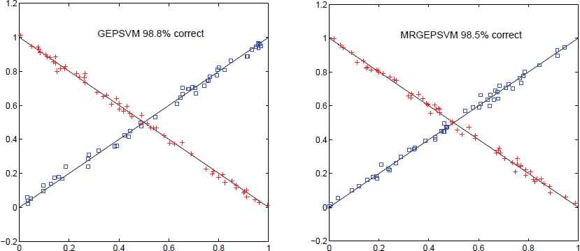
The “cross planes” learned by GEPSVM and MRGEPSVM together with their correctness on the training data set
5. Nonlinear MRGEPSVM
In this section, we extend our results to nonlinear classifiers. Suppose that the Euclidean space ℝn is mapped to a Hilbert space H, named as feature space instead of input space ℝn, through a nonlinear mapping function ϕ : ℝn → H. Let K(xi, xj) be kernel function in feature space satisfying K(xi, xj) = ϕ(xi)T ϕ(xj).The data samples A and B are mapped to ϕ(A) and ϕ(B), respectively. Let the fitting planes in feature space be denoted by:
Substituting (32) into (31), we obtain:
Similarly, by combining (33) with Tikhonov regularization, we obtain:
By an entirely similar argument, we can define an analogous minimization problem for the fitting plane of class 2.
After z1 and z2 are solved, two fitting planes in feature space are determined. In order to derive the decision rule in feature space, suppose we gave a new data point x ∈ ℝn to be classified. Then the distance between its image in feature space, i.e. ϕ(x), and the fitting plane of class 1, i.e. ϕ(xT) w1 + b1 = 0, is given by:
By using (32), (38) can be expressed as:
Similarly, the distance between and the fitting plane of class 2, i.e., ϕ(xT) w2 + b2 = 0, is given by:
The decision rule for nonlinear MRGEPSVM is the same as its linear version, expect the distances from x to fitting planes need to be calculated by (35) and (36) .
We now give an explicit statement for nonlinear MRGEPSVM algorithm.
Given m1 samples in ℝn represented by A ∈ ℝm1×n and m2 samples represented by B ∈ ℝm2×n.
|
Nonlinear Manifold Regularized Proximal Support Vector Machine via Generalized Eigenvalue
6. Experimental Results
To demonstrate the performance of the proposed method, we conducted experiments on several benchmark datasets from UCI Repository 27. Optimal values of all parameters involving each method were obtained by using a tuning set comprising of 10 percent of the data set. Table 1 shows the comparison of MRGEPSVM, TSVM, GEPSVM and SVM.
| MRGEPSVM | TSVM | GEPSVM | SVM | |
|---|---|---|---|---|
| Hepatitis | 85.16 ± 2.16 | 80.79 ± 3.74 | 58.29 ± 2.13 | 80.00 ± 2.03 |
| Ionosphere | 87.47 ± 3.38 | 88.03 ± 4.69 | 75.19 ± 3.43 | 86.04 ± 5.91 |
| Heart-statlog | 84.82 ± 1.98 | 84.44 ± 2.62 | 84.81 ± 3.11 | 84.07 ± 4.56 |
| Votes | 95.40 ± 1.62 | 96.08 ± 2.73 | 91.93 ± 3.08 | 94.50 ± 2.79 |
| Sonar | 79.81 ± 1.08 | 77.25 ± 3.75 | 66.76 ± 5.44 | 79.79 ± 2.13 |
| Pima | 74.88 ± 3.09 | 73.70 ± 5.14 | 74.60 ± 4.16 | 76.68 ± 3.82 |
Classification accuracy using linear kernel
From the experimental results listed in Table 1, we can see that MRGEPSVM gains superior performance than GEPSVM on nearly all datasets. We also performed experiments on several UCI datasets using RBF kernel. The performances of each method are shown in Table 2.
| MRGEPSVM | TSVM | GEPSVM | SVM | |
|---|---|---|---|---|
| Hepatitis | 81.94 ± 3.14 | 82.67 ± 5.03 | 78.25 ± 4.86 | 83.13 ± 3.56 |
| BUPA | 66.09 ± 2.71 | 67.83 ± 7.01 | 63.80 ± 3.25 | 58.32 ± 6.83 |
| WPBC | 79.72 ± 2.14 | 81.92 ± 4.17 | 62.70 ± 3.36 | 79.92 ± 3.16 |
Classification accuracy using nonlinear kernel
The aforementioned methods have been tested on benchmark data sets that are publicly available. Results regard their performance in terms of classification accuracy. The results regarding the linear kernel have been obtained using the first two repositories. The third one has been used in the non-linear kernel implementation. For each data set, the latter repository offers 100 predefined random splits into training and test sets. For several algorithms, results obtained from each trial, including SVMs, are recorded. Execution times and the other accuracy results have been calculated using an Intel Core i7 CPU 3.20 GHz, 8 GB RAM running Windows 8 with Matlab 2013b, during normal daylight operations. In the case of nonlinear kernel, we observe there are still perceptible improvements compared with GEPSVM. Meanwhile the accuracy of MRGEPSVM is close to TSVM and SVM. It seems that manifold structure didn’t greatly facilitate the performance in feature space. A possible explanation may lie in the higher dimensionality offset the effect brought by manifold structure within data samples after they are mapped.
Elapsed time are listed in Table 3 and Table 4, by different methods with Gaussian and linear kernel, respectively. In the linear one, MRGEPSVM and GEPSVM outperform TSVM and SVM in all cases. MRGEPSVM is at least twice faster than GEPSVM. When the Gaussian kernel is used, SVMs implementations achieve better performances with respect to the eigenvalues based methods. In all cases, MRGEPSVM is faster than GEPSVM.
| Dataset | MRGEPSVM | GEPSVM | TSVM | SVM |
|---|---|---|---|---|
| Votes | 1.1473 | 5.8744 | 0.4523 | 0.2022 |
| Sonar | 3.8717 | 5.8947 | 0.1543 | 0.4080 |
| Pima | 0.0296 | 0.1143 | 0.0302 | 7.1968 |
| Flare-solar | 1.9839 | 16.1654 | 2.1429 | 4.4562 |
| Waveform | 0.5998 | 4.480 | 0.9016 | 0.2284 |
| Thyroid | 0.0246 | 0.1280 | 0.0503 | 0.0718 |
| Heart | 0.0361 | 0.2187 | 0.0278 | 0.1732 |
| Banana | 0.4989 | 3.1102 | 0.0346 | 1.3505 |
| Breast-cancer | 0.0688 | 0.3544 | 0.0429 | 0.1188 |
Elapsed time in seconds using Gaussian kernel
| Dataset | MRGEPSVM | GEPSVM | TSVM | SVM |
|---|---|---|---|---|
| Votes | 0.0119 | 0.0277 | 0.0024 | 0.0019 |
| Sonar | 0.0364 | 0.0854 | 0.0589 | 0.0395 |
| Pima | 0.0015 | 0.2858 | 0.6809 | 0.0013 |
| Flare-solar | 0.0158 | 0.1673 | 0.1092 | 0.0893 |
| Waveform | 0.0013 | 0.0934 | 0.0438 | 0.0472 |
| Thyroid | 0.0011 | 0.0183 | 0.00524 | 0.0018 |
| Heart | 0.0012 | 0.1091 | 0.0019 | 0.0011 |
| Banana | 0.0024 | 0.1578 | 0.0063 | 0.0038 |
| Breast-cancer | 0.0002 | 0.0158 | 0.0016 | 0.0009 |
Elapsed time in seconds using linear kernel
USPS database is a handwritten numeral recognition database provided by the United States postal service, which includes 10 kinds of gray images from 0 to 9, where the gray value has been normalized, with each figure containing 1100 images of 16 × 16 pixels. Table 5 is the average accuracy and standard deviation of different algorithms using USPS dataset.
| Num. | SVM Test±Std (%) | LPP Test±Std (%) | TSVM Test±Std (%) | GEPSVM Test±Std (%) | MRGEPSVM Test±Std (%) |
|---|---|---|---|---|---|
| l = 10 | 77.14 ± 1.97 | 82.26 ± 1.73 | 81.12 ± 1.67 | 81.41 ± 1.85 | 82.26 ± 1.37 |
| l = 20 | 84.67 ± 0.93 | 89.19 ± 1.00 | 89.40 ± 1.09 | 87.78 ± 1.34 | 89.97 ± 1.06 |
| l = 30 | 86.07 ± 1.62 | 91.60 ± 1.07 | 91.93 ± 0.87 | 90.51 ± 1.13 | 92.99 ± 0.98 |
| l = 40 | 88.13 ± 1.13 | 93.22 ± 1.02 | 93.49 ± 0.95 | 91.88 ± 0.99 | 94.33 ± 0.93 |
| l = 50 | 90.48 ± 1.34 | 94.50 ± 0.88 | 94.46 ± 1.05 | 93.40 ± 1.26 | 95.50 ± 1.08 |
The average accuracy and standard deviation of different algorithms in USPS dataset
In this experiment, we randomly selected 110 image data sets from each class of samples, and randomly selected 10% and 20% of the data as the training set to verify the MRGEPSVM algorithm. The penalty parameters C of SVM and TWSVM, as well as the regularization terms of MRGEPSVM and GEPSVM, are selected from the collection {2i| − 9,…, 9}. The value k of KNN is selected from the collection {3, 4,…,20}.
The experimental set-up is meant to simulate a real-world situation: we considered binary classification problems due to the splits of the training data, where all of one driver cases were labeled and all the rest were left unlabeled. The test set is composed of entirely new drivers, forming the separate group.
In Fig. 6, we compare the error rates of 30 binary classification problems of GEPSVM, MRGEPSVM algorithm. We train on the same driver from a training set of examples, and test on the remaining five set of samples. We considered the task of classifying the driver whether he meets obstacles as a binary classification problem.
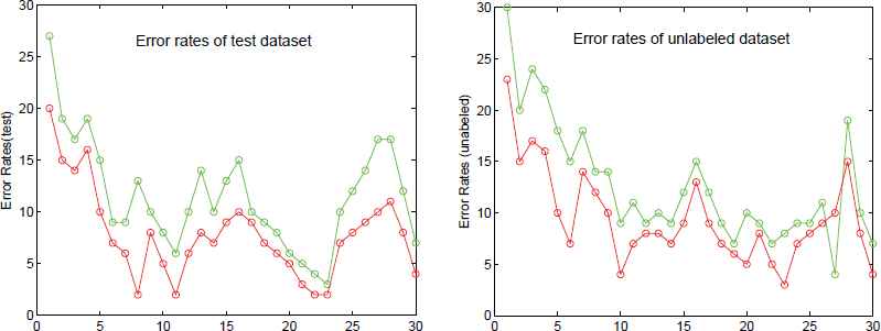
Error rates of 30 binary classification problems
7. Conclusions
In this paper, a novel proximal support vector machine, called manifold regularized GEPSVM, is presented. Our analysis allows us to see the role of manifold regularization in proximal support vector machine via generalized eigenvalue in a clear way. MRGEPSVM is derived by designing a modified locality preserving projections criteria and incorporating it into GEPSVM. Unlike conventional LPP, we project the data points onto planes and require the local geometry structure to be preserved. In GEPSVM, we also solve a pair of eigenvalue problems to determine the two fitting planes. One advantage of MRGEPSVM is that it demonstrates that manifold regularization is suitable for GEPSVM and its variants. As to future work, we believe the proposed regularization technique may be applied in more powerful classifiers, e.g. Twin SVM, to further boost its performance.
Acknowledgements
This work is partially supported by the National Natural Science Foundation of China (Grant U1564201, No. 51108209, No. 50875112, No. 61573171 and No. 70972048), the Natural Science Foundation of Jiangsu Province (Grant No. BK2010339 and No. BK20140570), the Natural Science Foundation of the Jiangsu Higher Education Institutions of China (Grant No. 10KJD580001), the College Graduate Research and Innovation Program of Jiangsu Province(Dr. Innovation) (Grant No. CXLX11 0593), the Project Funded by the Priority Academic Program Development of Jiangsu Higher Education Institutions(PAPD), the Project Funded by the department of transport information (Grant 2013-364-836-900), the “Six Talent Peak” project in Jiangsu Province (DZXX-048), and the National Statistical Science Research Project (2014596).
References
Cite this article
TY  - JOUR
AU  - Jun Liang
AU  - Fei-yun Zhang
AU  - Xiao-xia Xiong
AU  - Xiao-bo Chen
AU  - Long Chen
AU  - Guo-hui Lan
PY  - 2016
DA  - 2016/12/01
TI  - Manifold Regularized Proximal Support Vector Machine via Generalized Eigenvalue
JO  - International Journal of Computational Intelligence Systems
SP  - 1041
EP  - 1054
VL  - 9
IS  - 6
SN  - 1875-6883
UR  - https://doi.org/10.1080/18756891.2016.1256570
DO  - 10.1080/18756891.2016.1256570
ID  - Liang2016
ER  -