
Flower Pollination Algorithm for Multimodal Optimization
- DOI
- 10.2991/ijcis.2017.10.1.42How to use a DOI?
- Keywords
- Flower Pollination Algorithm; Multimodal optimization; Multimodal Flower Pollination Algorithm
- Abstract
This paper proposes a new algorithm called Multimodal Flower Pollination Algorithm (MFPA). Under MFPA, the original Flower Pollination Algorithm (FPA) is enhanced with multimodal capabilities in order to find all possible optima in an optimization problem. The performance of the proposed MFPA is compared to several multimodal approaches considering the evaluation in a set of well-known benchmark functions. Experimental data indicate that the proposed MFPA provides better results over other multimodal competitors in terms of accuracy and robustness.
- Copyright
- © 2017, the Authors. Published by Atlantis Press.
- Open Access
- This is an open access article under the CC BY-NC license (http://creativecommons.org/licences/by-nc/4.0/).
1. Introduction
In optimization1, the idea is to find an acceptable solution within a feasible search space guided by the values of an objective function. Optimization problems comprises many areas as engineering, medicine, economics, just to mention a few2. The problem of optimization has been commonly solved through the use of deterministic methods such the Gradient descent algorithm3 and the Levenberg -Marquardt method4. These techniques provide a theoretical guarantee of finding the global optimum assuming some theoretical suppositions about objective function such as the unimodality5,6. However, most of the practical optimization problems tend to generate multimodal surfaces maintaining several local and global optima7. Under such conditions, the use of classical methods faces great difficulties in finding an acceptable solution due the existence of several optima in the objective function.
As an alternative to deterministic techniques, the problem of optimization has also been conducted through Evolutionary Computation Techniques (ECT)8 . Such approaches are inspired by our scientific understanding of biological or social systems, which at some level of abstraction can be conceived as optimization processes. ECT have been developed by a combination of deterministic rules and randomness to mimic the behavior of natural or social entities. Different to deterministic methods, under the ECT perspective, the existence of several global and local optima does not represent a difficulty due to its search properties. Recently, several ECT have been proposed with interesting results. These methods involves the well-known Genetic Algorithm (GA) proposed by Holland9 and Goldberg10, Evolutionary Programming (EP) proposed by Rechenberg11 and the Differential Evolution (DE) developed by Storn and Price12 and Particle Swarm Optimization (PSO) method introduced by Kennedy & Eberhart13. Other ECT metaphors considers the emulation of physical phenomena such Simulated Annealing (SA) proposed by Kirkpatrick14, the Electromagnetism-like Optimization (EMO) developed by Birbil and Fang15, and the Gravitational Search Algorithm (GSA) proposed by Rashedi16. The interaction among animals and their ecosystems has also used as optimization metaphors such the Particle Swarm Optimization developed by Kennedy and Eberhart17, the Artificial Bee Colony optimization (ABC) developed by Karaboga18 and the Cuckoo Search method (CS) proposed by Yang19.
Most of research work on ECT has been accomplished for locating the global optimum. However, the acquisition of multiple promissory solutions is especially useful in engineering, since the best solution may not always be realizable due to several realistic constraints. Therefore, from a practical point of view, it is desirable to identify and maintain all the possible optima solutions through the overall optimization process. The process of finding the global optimum and multiple local optima is known as multimodal optimization20. ECT perform well for locating a single optimum with remarkable performance but fail to provide multiple solutions. The process of locating all the optima in a single run is more complicated than global optimization. Detection and maintenance of multiple solutions are two crucial processes in ECT for solving multimodal optimization problems since they are originally devised to find only a global solution.
Several schemes have been incorporated into the original ECT to make them suitable for registering and maintaining potential optima. Some approaches include the Crowding method proposed by Jong21. In Crowding, the main objective is to preserve diversity replacing similar individuals by individuals of better quality. Based on this approach, several multimodal algorithms have been designed considering different evolutionary methods such as the Crowding Differential evolution (CDE)22,23 and Deterministic Crowding Genetic Algorithms (DCGA)24,25.
Fitness sharing is other multimodal scheme introduced by Goldberg and Richardson26. In fitness sharing, a function diminishes the fitness values of similar solutions, so that they have a lower probability to be selected in the new population27,28. This method has produced several multimodal algorithms such as the Fitness Sharing Differential Evolution (FSDE)22.
On the other hand, speciation-based niching methods are multimodal techniques which require the partition of the complete population into different sub-populations considered as species. Some multimodal algorithms of this category include the distance-based locally informed PSO29, the Ensemble Speciation (ES)30 and the History-based Topological speciation31.
The above multimodal techniques have been applied to original ETC in order to produce their multimodal extensions. However, other researchers have designed several evolutionary computation algorithms with multimodal capacities. Such methods use as inspiration our scientific understanding of biological systems, which at some level of abstraction can be represented as multimodal optimization processes. Some examples of these methods include the Clonal Selection Algorithm32, the Multimodal Gravitational Search algorithm (MGSA)33 and the Region-Based Memetic method (RM)34. Such approaches employ operators and structures which support the finding and maintaining of multiple-solutions.
On the other hand, the Flower Pollination Algorithm (FPA)35 is a recent evolutionary computation algorithm which is inspired on the natural pollination flower concept. Different to the most of existent evolutionary algorithms, FPA presents a better performance in multimodal problems, avoiding critical flaws such as the premature convergence to sub-optimal solutions. FPA considers both exploration and exploitation stages through the entire optimization process. For the exploration stage, FPA considers the Lévy flights36 rather than simple random walks to discover new candidate solutions through the entire feasible region. For the exploitation stage, FPA considers the flower constancy which models the pollinator tendency to pollinate certain kind of flowers giving a reproduction probability in order to increase the pollination efficiency. As a result, FPA is potentially far more efficient than other ECT causing its election to incorporate multimodal capabilities extending its operands. Such characteristics have motivated its use to solve an extensive variety of engineering applications37,38.
This paper presents a new multimodal optimization algorithm called Multimodal Flower Pollination Algorithm (MFPA). The method combines the FPA algorithm with three elements that allow the operation of several optima. The first element involves a memory mechanism39 which allows an efficient registering of potential local optima according to their fitness value and the distance to other potential solutions. The second element aims to accelerate the detection process of potential local minima. The original FPA search strategy is mainly conducted by the best individual found so-far (global optimum). Under the second element, the FPA strategy is modified to be influenced by individuals that are contained in the memory mechanism. The third element is a depuration procedure to eliminate similar solutions that possibly represent the same optimum. Numerical simulations have been conducted on fourteen benchmark functions to show the effectiveness of the proposed scheme. The performance of the proposed MFPA is compared to the results obtained by four multimodal algorithms: CDE, FSDE, DCGA and CSA. Experimental results indicate that the proposed MFPA is capable of providing better and even more consistent optima solutions over their well-known multimodal competitors for the majority of benchmark functions.
The paper is organized as follows: Section 2 describes the original Flower Pollination Algorithm (FPA). Section 3 presents the proposed MFPA. Section 4 presents the experimental results obtained. Finally, Section 5 establishes some conclusions.
2. Flower Pollination Algorithm (FPA)
Flower Pollination Algorithm has been recently developed by Yang35. FPA is based on the pollination process of flowers. The flower pollination process aims to the transfer of pollen between the same flower or other flowers within the same or different plant for their reproduction. Pollination can be carried out by the so-called pollination vectors like birds, insects, honey bees and other animals or by water, wind, light etc.; making the pollination process be divided in two different ways; biotic and abiotic.
Biotic pollination is the most common type of flower pollination and constitutes the 90% of the total natural pollination around the world. This kind of pollination requires intervention of agents such insects to transfer pollen through flowers of different plants. The mechanism to accomplish biotic pollination by terms of these agents is called cross-pollination also known as allogamy and occurs when pollen is delivered to a flower from a different plant. On the other hand, abiotic pollination refers to situations where non-living organisms like water and wind transfer pollen. Only 10% of the world total natural pollination belongs to this pollination category and it could be accomplish by self-pollination. Self-pollination occurs when pollen is delivered to flowers of the same plant by non-living agents extending the way flower reproduction takes place.
In the biological process of flower pollination an important behavior occurs between flowers and the foraging stage of the pollinators. This behavior is known as flower constancy and mimics the biological phenomenon that a pollinator tend to visit certain flower species while passing by other flower species through their travel in order to improve the pollination process for reproduction.
The Natural flower pollination process analogy is used to develop the FPA algorithm. Additionally, this algorithm use the so-called Lévy flights36 rather than simple random walks to enhance the exploration area within the search space. Biological processes are difficult to be modeled as evolutionary algorithms. Simplification of biological processes is necessary for successful implementation as evolutionary algorithm. The FPA algorithm simplifies the natural flower pollination process into four idealized rules as follows:
- (i)
Global Pollination Rule: Biotic in terms of cross-pollination is considered as a global pollination operation with pollinators performing flights through flowers. This rule can be formulated as the exploration step that simulates global search through the search space in terms of Lévy flights.
- (ii)
Local Pollination Rule: Abiotic in terms of self-pollination is considered as a local pollination operation and could be modeled as the exploitation stage to guide the search to find better solutions.
- (iii)
Reproduction Probability Rule: This rule can be considered as the flower constancy behavior which models the pollinator tendency to pollinate certain kind of flowers giving a reproduction probability in order to increase the pollination efficiency.
- (iv)
Switch Probability Rule: This rule acts like an operator that controls the switching process between global and local pollination in the evolution process and it is defined as sp ∈ [0,1].
In the real world, each plant can have many flowers and each of them produce millions of pollen gametes. From the implementation point of view, the FPA considers only one flower that produces only one pollen gamete. In the FPA, a population
The four idealized rules described before could be implemented into three basic operations for successful implementation of the evolutionary process for the FPA: Global Pollination through Lévy flights, Local Pollination considering flower constancy and Elitist Selection.
2.1 Global pollination through lévy flights
In the global pollination step, pollen is carried by living agents who travel through Lévy flights all over the search space. Lévy flights enhance exploration stage within the search space rather than simple random walks. They represent one on the most powerful operators in FPA and they mimic the peculiar behavior that living agents travel long distance in order to carry pollen to flowers. The Lévy distribution that describes the travel for the pollinators is defined as:
Once si has been calculated, the position perturbation is obtained by:
2.2 Local pollination considering flower constancy
This operation mimics the flower constancy behavior between a pollinator and the similarity between flower species and can be represented as:
2.3 Elitist selection
After obtained a new candidate solution
This operation specifies that only high-quality solutions remains and provide the development of next generation through the best optima solution for the optimization problem to be solved. The complete pseudocode for the FPA implementation is shown in Fig 1.

The Flower Pollination Algorithm Pseudocode.
3. Multimodal Flower Pollination Algorithm (MFPA)
In FPA, the biological flower pollination process is simplified in order to be implemented as an evolutionary algorithm. An individual
This multimodal adaptation incorporates three new operators proposed by Cuevas and Reyna-Orta39. The first operand is the utilization of a memory mechanism to identify potential local and global optima. The second operand is the adaptation of new selection strategy instead of the well-known elitist selection to ensure solution diversity. And the last operation considers a mechanism to depurate the memory mechanism to cyclically eliminate duplicated solutions. These three new operators for the proposed MFPA are performed during the evolutionary process that is divided into three states.
The first state s=1 corresponds from 0 to 50% of the total evolutionary process. The second state s=2 involves 50 to 90%. And the third state s=3 belongs 90 to 100%. The reason this division of the evolutionary process is implemented is that the proposed method can be capable of act according on the current state of the evolutionary process. The following sections describe the three new adaptations to provide multiple optima localization in the original FPA. These operators are Memory Mechanism (MM), Selection Strategy (SS) and Depuration Procedure (DP).
3.1 Memory mechanism (MM)
Within MFPA, a population
In multimodal optimization, both global and local optima describe two important features in order to be identified: they have significant good fitness value and they represent the best fitness in a certain neighborhood. Therefore the necessity to efficiently register potential global and local optima including these features should be implemented into a memory mechanism considering the past and new solutions in the overall evolutionary process.
The memory mechanism constitutes an array of M={m1, m2, …, mg} elements where each memory element mw defines potential global or local optimum that fulfills the optima features described before and corresponds a d-dimensional vector {mw,1, mw,2, …, mw,d} where each dimension corresponds to a decision variable. Therefore, a memory element is considered a solution to the optimization problem to be solved. To accomplish a successful registration in the memory, the memory mechanism occurs in two different phases: initialization and capture. Initialization phase is applied only once within the optimization process. That is, when k=0 only the best flower solution xbest of the initial population xk is successful register into the memory due to the good fitness value and its representation as the best individual in a certain neighborhood. Once the initialization phase is complete, the memory mechanism becomes more interesting and it is described by the next section.
3.1.1 Capture phase
This phase is applied from the first iteration k=1 to the last iteration s=1 at the end of the global or the local pollination operations in the entire evolutionary process. At this stage, each solution xi that corresponds to potential global or local optima is registered as memory element mw if it has a good fitness value and it is the best individual in a determined neighborhood. In order to register a solution into the memory. xi must be tested considering two rules: significant fitness value and non-significant fitness value rule.
Significant Fitness Value Rule
This rule compares the fitness value of the solution
To implement the significant fitness value rule, the normalized distance ||Di,g|| between the
And the acceptance probability function P(||Di,g||, s) is defined according to the nearest memory element mn such as:

The Significant Fitness Value Rule Pseudocode.
Non-Significant Fitness Value Rule
This rule is the counterpart of the significant value rule, the difference that this rule performs within the evolutionary process is to capture potential local optima with low fitness values. The operation of this rule considers a solution
Therefore, the probability P assigns a probability greater than zero to solutions that have good fitness values. In order to test if a solution

The Non-Significant Fitness Value Rule Pseudocode.
3.2 Selection strategy (SS)
This operation extends the elitist selection strategy used not only in the original FPA but also in many evolutionary algorithms reported in the literature such as Particle Swarm Optimization13, Differential Evolution12, Gravitational Search Algorithm16 and Cuckoo Search19, just to mention few of them. Elitist selection considers only the best individuals to prevail through the overall evolutionary process41. This common selection strategy does not provide a mechanism to maintain potential solutions and treat them as global or local minima. Therefore elitist selection strategy must be change in order to perform multimodal optimization. MFPA implements a new selection strategy that allows capturing potential global and local minima optima. The SS is performed just at the end of the MM operation.
By the new selection strategy, the new population xnew is generated considering the first n elements of the memory being n the size of the initial population. An interesting point in the memory mechanism is the fact that each of its elements is considered as a minimum solution being the first n elements the best solutions that describe global or local features. The selection strategy complements the powerful operation of the memory mechanism by replacing each individual of the original population by each element of the memory keeping the population diversity through the evolutionary process. In case the number of elements inside the memory is less than n, the remaining individuals n – g are the best individuals of the original population xk. The procedure to implement this selection strategy is resumed in Fig 4.

The Selection Strategy Pseudocode.
3.3 Depuration procedure (DP)
Elitist selection considers only the best individuals to prevail during the evolutionary process. Therefore this classical approach is not appropriate for multimodal optimization. In multimodal optimization a new selection strategy must be defined in order to capture multiple optima solutions in a single execution42. Some approaches for this capability include the well-known Deterministic Crowding and Fitness Sharing 43 techniques. However these techniques generate a final solution set as the same size of the initial population causing individual concentrations in the final solutions. In MFPA the new selection strategy (SS) allows multiple optima registration each iteration through the overall evolutionary process inside the memory. However each individual allocated inside the memory could represent the same minimum. The depuration procedure in MFPA eliminates similar individuals inside the memory improving the detection of significant and valid solutions. The execution of this depuration stage occurs just at the end of each state s.
The memory mechanism of MFPA tends to allocate several solutions over the same minimum. The depuration procedure finds the distances among concentrations and eliminates solutions that are similar to each other in order to improve the search using only the most significant solutions. The procedure consists of taking the best element mbest inside the memory and calculates all the distances among each of the memory elements mr. Later, test the fitness value of the medium point between mbest and mr in order to find a depuration ratio that allows elimination of all nearest solutions to mbest. Then if the fitness value of the medium point J((mbest + mr)/2) is not worse than J(mbest) and J(mr), the element mr is considered part of the same concentration of mbest. However, if the fitness value of the medium point J((mbest + mr)/2) is worse than J(mbest) and J(mr), then mr is considered part of another concentration. If the last situation occurs, the distance between mbest and mr can be considered as a maximum depuration ratio distance which will be used to eliminate solutions within a certain neighborhood. The calculation of the depuration ratio Drt takes the 85% of the maximum distance between mbest and mr and is defined as:
The implementation of this depuration procedure is resumed in Fig 5.

The Depuration Procedure Pseudocode.
3.4 Complete multimodal flower pollination algorithm
In MFPA three new operations are added to the original FPA in order to incorporate multimodal capacities. This new operations consist of capturing potential optima solutions through the overall evolutionary process maintaining only the individuals which have significant fitness value and the ones that represents the best in a certain neighborhood. The first operation to incorporate multimodal capacities is based on a memory mechanism which allows multiple registrations of individuals in a single execution. The second operation is a new selection strategy which does not select only the best individual through the process but also a set of solutions that present global or local minima features. The last operation of the implementation of MFPA is the inclusion of depuration procedure for the memory storage. In classical multimodal approaches the final solution set has the same size of the initial population due the multiple solution registration. This entails the generation of minima concentration in a certain neighborhood. In order to eliminate these concentrations to keep only the best individual of each of them, the depuration procedure of MFPA considers a depuration ratio between each element of the memory and the remaining elements inside the memory. Later, all the elements inside within an area determined by the depuration ratio will be eliminated allowing significant solutions to prevail. The complete pseudocode for MFPA implementation with this three operations is resumed in Fig 6.
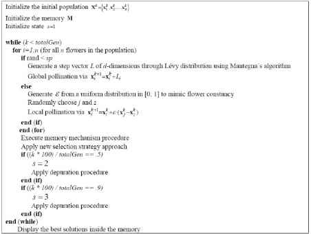
The Multimodal Flower Pollination Algorithm Pseudocode.
4. Experimental Results
This section presents the performance of MFPA over a set of 2D benchmark functions in order to compare the minima solutions of the proposed MFPA against other multimodal algorithms. The Section 4.1 describes the performance criteria used in order to evaluate the results obtained by MFPA against the results of four algorithms commonly used in multimodal optimization comparing them with five different performance indexes. The Section 4.2 reports the approach used in order to determine the true optima set per function will be considered to calculate each of the five indexes. Finally, the Section 4.3 reports the results obtained for MFPA compared to each of the four algorithms according to the performance indexes criteria using a set of fourteen benchmark functions.
4.1 Performance criteria
This section describes a set of five performance indexes commonly used to evaluate the performance of multimodal algorithms23,39,44. The first index used is the Effective Peak Number (EPN) which expresses the amount of detected peaks. The second index is the Maximum Peak Ratio (MPR) to evaluate the quality of the solutions over the true optima. The third index is Peak Accuracy (PA) which calculates the total error produced among the identified solutions and the true optima. The fourth index calculated is the Distance Accuracy (DA) to measure the error produced by the components between identified solutions and true optima. And the last index, the Number of Function Evaluations (NFE) shows the total number of function calculations of each algorithm through the experiment. Each of these indexes is formally defined as follows.
The Effective Peak Number (EPN) expresses the quantity of valid detected peaks. That is, each solution of each algorithm is considered as an optimum oi if the distance between the solution wj and the true optima oi is not greater than 0.05. That is, only the 5% of error is permitted for each solution wj against its correspondent true optima oi. The EPN is resumed as:
PA only takes the error based on the fitness value for the true optima against the identified optima but not considers if the peak of oi and wi are close. Under such circumstance, the Distancy Accuracy is calculated to consider the peak closeness and it is calculated as follows:
The last index used for the evaluation of the performance benchmark is the Number of Function Evaluations which calculates the total number of function calculations in order to obtain a set of final solutions for each algorithm.
4.2 True optima determination
In order to calculate these performance indexes, a set of fourteen benchmark functions with different complexities is proposed. Due the fact these performance indexes operate among identified optima and true optima values for each benchmark function, the necessity to propose true optima values is essential. In the reported literature, does not exist selection criteria for true optima to test the performance indexes. Therefore a consideration to take true optima values must be done. In this study, all the optima found below the medium point of the highest and lowest values in each function will be considered as true optima for minimization problem. That is, obtaining the medium point of the highest and lowest function values, a set of true optima values will be determined as follows:
4.3 Performance results
To compare the results of the MFPA using the performance indexes described in Section 4.1, a comprehensive set of 14 multimodal functions, collected from Refs. 45, 46, has been used. Table 1 presents the benchmark functions J1 – J14 considered in our experimental study. In Table 1, it is exposed the characteristics of each function such as the number of optima and the search space domain. The experiments compare the performance of MFPA against the Fitness Sharing Differential Evolution (FSDE), the Crowding Differential Evolution (CDE), the Clonal Selection Algorithm (CSA), the Deterministic Crowding Genetic Algorithm (DCGA), the Region-Based Memetic method (RM)34, the Multimodal Gravitational Search algorithm (MGSA)33 and the Ensemble Speciation DE (ES)30. For all the algorithms the population size is set to 50 individuals and the number of total iterations has been set to 500.
| Function | Search Domain | Optima Number |
|---|---|---|
| Bird | [−2π, 2π] | 6 |
|
|
||
| Test Tube Holder | [−10, 10] | 4 |
|
|
||
| Penholder | [−11, 11] | 12 |
|
|
||
| Rastriguin | [−5.12, 5.12] | 21 |
|
|
||
| Himmelblau | [−6, 6] | 5 |
|
|
||
| Six Hump Camel | x1 = [–3, 3] x2 = [–2, 2] |
3 |
|
|
||
| Giunta | [−1, 1] | 4 |
|
|
||
| Rastriguin49 | [−1, 1] | 8 |
|
|
||
| Roots | [−2, 2] | 6 |
|
|
||
| Vincent | [0.25, 10] | 36 |
|
|
||
| Multi Peak | [−2, 2] | 40 |
|
|
||
| Alpine 02 | [0, 10] | 8 |
|
|
||
| Cosine Mixture | [−1, 1] | 12 |
|
|
||
| Egg Crate | [−5, 5] | 9 |
|
|
Benchmark functions J1 – J14 of our experimental study
The parameter setting used in the comparison is described below. For the case of the FSDE method, the following parameters have been used: the variant implemented is DE/rand/bin22 where crossover probability cr=.9, differential weight dw=0.1 with sharing radius σshare = 0.1 and α=1.0 according to Ref. 39. With regard to the CDE algorithm, its configuration has been assumed with: the variant implemented is DE/rand/bin where crossover probability cr=.9, differential weight dw=0.1 with crowding factor cf=50. Using the guidelines of Ref. 39. In case of the DCGA method, it has been implemented following the following guidelines: a crossover probability cp=0.9 and a mutation probability mp=0.1 using roulette wheel selection. The CSA has been set as follows: the mutation probability mp=0.01, the percentile to random reshuffle per=0.0 and the clone per candidate fat=.1. In case of the proposed MFPA, the probability switch between Global and Local Pollination is set to sp=.25. In the experiments, all the remaining methods, RM34, MGSA33 and ES30 have been configured according to their own reported guidelines.
The performance results among the algorithms are reported in Tables 2 and 3. For the sake of clarity, they are divided in two groups, Table 2 for functions J1 – J7 and Table 3 for functions J8 – J14. Both Tables register the performance indexes with regard to the effective peak number (EPN), the maximum peak ratio (MPR), the peak accuracy (PA) and the distance accuracy (DA).
| Function | Algorithm | EPN | MPR | PA | DA | NFE |
|---|---|---|---|---|---|---|
| J1 | FSDE | 2.6600 (0.7174) | 0.7540 (0.1914) | 91.0354 (66.1408) | 16.1303 (2.8272) | 2.5000e+04 (0.0000) |
| CDE | 5.9800 (0.1414) | 1.0017 (0.0006) | 0.5970 (0.2103) | 0.3427 (1.0932) | 2.5000e+04 (0.0000) | |
| CSA | 1.0000 (0.0000) | −0.0043 (0.0000) | 350.1699 (0.0000) | 26.0224 (0.0015) | 1.0020e+03 (0.0000) | |
| DCGA | 0.4200 (0.5379) | 0.1222 (0.1617) | 309.4281 (55.7500) | 25.3591 (2.2885) | 1.3850e+06 (288.1563) | |
| RM | 5.2800 (0.6402) | 0.7036 (0.1274) | 107.5283 (43.2990) | 8.3606 (3.8876) | 5.0100e+02 (0.0000) | |
| MGSA | 1.0000 (0.0000) | −0.0237 (0.0845) | 359.8525 (29.1997) | 26.2039 (1.2992) | 2.5000e+04 (0.0000) | |
| ES | 2.5000 (0.6145) | 0.7698 (0.1923) | 409.6047 (53.8922) | 24.4823 (0.6759) | 1.1941e+05 (37170.0853) | |
| MFPA | 5.3600 (0.4849) | 1.0044 (0.0021) | 1.5166 (0.7206) | 0.8587 (0.5105) | 2.5203e+04 (11.4375) | |
| J2 | FSDE | 2.8000 (1.2936) | 0.6869 (0.3166) | 13.5855 (13.7374) | 4.7114 (4.3008) | 2.5000e+04 (0.0000) |
| CDE | 3.5400 (0.8621) | 0.8853 (0.2156) | 5.0055 (9.3480) | 1.7228 (2.9999) | 2.5000e+04 (0.0000) | |
| CSA | 0.0000 (0.0000) | 0.0000 (0.0000) | 43.3904 (0.0000) | 14.0472 (0.0000) | 1.0020e+03 (0.0000) | |
| DCGA | 0.2200 (0.4185) | 0.0550 (0.1046) | 41.0050 (4.5371) | 13.2824 (1.4547) | 1.3850e+06 (285.0152) | |
| RM | 3.7400 (0.4431) | 0.7180 (0.1452) | 12.2383 (6.3022) | 3.3264 (1.5125) | 5.0100e+02 (0.0000) | |
| MGSA | 0.9200 (0.2740) | 0.0984 (0.0758) | 39.1188 (3.2869) | 13.9158 (0.9773) | 2.5000e+04 (0.0000) | |
| ES | 2.4400 (1.0910) | 0.6100 (0.2744) | 16.9892 (11.8235) | 12.7849 (2.4176) | 1.2220e+05 (36883.9504) | |
| MFPA | 3.7800 (0.5067) | 0.9454 (0.1267) | 2.4043 (5.4939) | 0.8865 (1.7634) | 2.5165e+04 (11.3026) | |
| J3 | FSDE | 5.0400 (1.5381) | 0.4226 (0.1285) | 6.5307 (1.4539) | 84.2616 (19.0553) | 2.5000e+04 (0.0000) |
| CDE | 7.7000 (2.6973) | 0.6433 (0.2242) | 4.0347 (2.5359) | 51.9124 (32.6811) | 2.5000e+04 (0.0000) | |
| CSA | 0.0000 (0.0000) | 0.0000 (0.0000) | 11.3110 (0.0000) | 147.5853 (0.0000) | 1.0020e+03 (0.0000) | |
| DCGA | 0.0000 (0.0000) | 0.0000 (0.0000) | 11.3110 (0.0000) | 147.5853 (0.0000) | 1.3850e+06 (280.2022) | |
| RM | 10.1600 (1.0947) | 0.6011 (0.1735) | 4.5117 (1.9619) | 32.1361 (12.1145) | 5.0100e+02 (0.0000) | |
| MGSA | 0.2400 (0.4314) | 0.0103 (0.0217) | 11.1949 (0.2450) | 145.6805 (3.4615) | 2.5000e+04 (0.0000) | |
| ES | 0.0000 (0.0000) | 0.0000 (0.0000) | 11.3110 (0.0000) | 147.5853 (0.0000) | 8.5205e+04 (23788.6955) | |
| MFPA | 11.6400 (0.6928) | 0.9700 (0.0577) | 0.3398 (0.6531) | 4.8550 (8.5080) | 2.5175e+04 (11.9867) | |
| J4 | FSDE | 1.0000 (0.0000) | 0.0146 (0.0204) | 71.6704 (0.9852) | 34.4840 (0.5887) | 2.5000e+04 (0.0000) |
| CDE | 15.4000 (2.8067) | 0.6803 (0.1438) | 24.1608 (10.5013) | 10.1389 (4.9194) | 2.5000e+04 (0.0000) | |
| CSA | 1.0000 (0.0000) | 0.0000 (0.0000) | 72.3042 (0.0000) | 35.0906 (0.0000) | 1.0020e+03 (0.0000) | |
| DCGA | 1.0600 (0.3136) | 0.0011 (0.0062) | 72.2399 (0.3372) | 35.0315 (0.3091) | 1.3850e+06 (307.9098) | |
| RM | 9.9600 (2.6570) | 1.2543 (0.7687) | 90.0817 (47.8586) | 29.9317 (2.0631) | 5.0100e+02 (0.0000) | |
| MGSA | 1.0000 (0.0000) | 0.3463 (0.1663) | 96.4085 (12.0253) | 37.4041 (0.9597) | 2.5000e+04 (0.0000) | |
| ES | 21.0000 (0.0000) | 0.4219 (0.3969) | 51.4849 (12.4425) | 40.8538 (5.3202) | 1.2057e+05 (39344.2203) | |
| MFPA | 19.5000 (1.1294) | 0.8826 (0.0538) | 8.4881 (3.8911) | 2.5735 (1.8889) | 2.5241e+04 (16.7986) | |
| J5 | FSDE | 1.0000 (0.0000) | 0.3181 (0.0091) | 4526.5866 (60.4546) | 29.2162 (0.0624) | 2.5000e+04 (0.0000) |
| CDE | 5.0000 (0.0000) | 1.0000 (0.0000) | 0.0085 (0.0000) | 0.0228 (0.0002) | 2.5000e+04 (0.0000) | |
| CSA | 0.0000 (0.0000) | 0.0000 (0.0000) | 6638.3536 (0.0000) | 37.6246 (0.0000) | 1.0020e+03 (0.0000) | |
| DCGA | 0.0000 (0.0000) | 0.0000 (0.0000) | 6638.3536 (0.0000) | 37.6246 (0.0000) | 1.3850e+06 (315.5938) | |
| RM | 4.9600 (0.1979) | 0.9795 (0.0404) | 136.0493 (268.3073) | 1.3495 (1.3138) | 5.0100e+02 (0.0000) | |
| MGSA | 0.5600 (0.5014) | 0.0080 (0.0108) | 6585.5431 (71.8419) | 36.1061 (1.6747) | 2.5000e+04 (0.0000) | |
| ES | 0.0000 (0.0000) | 0.0000 (0.0000) | 6638.3536 (0.0000) | 37.6246 (0.0000) | 3.6959e+04 (464.7521) | |
| MFPA | 5.0000 (0.0000) | 1.0000 (0.0000) | 0.0085 (0.0000) | 0.0229 (0.0006) | 2.5113e+04 (7.4773) | |
| J6 | FSDE | 3.0000 (0.0000) | 0.9337 (0.0415) | 31.5887 (19.7709) | 0.3095 (0.2098) | 2.5000e+04 (0.0000) |
| CDE | 3.0000 (0.0000) | 1.0000 (0.0000) | 0.0000 (0.0000) | 0.0000 (0.0000) | 2.5000e+04 (0.0000) | |
| CSA | 0.0000 (0.0000) | 0.0000 (0.0000) | 476.7000 (0.0000) | 10.8167 (0.0000) | 1.0020e+03 (0.0000) | |
| DCGA | 0.0000 (0.0000) | 0.0000 (0.0000) | 476.7000 (0.0000) | 10.8167 (0.0000) | 1.3850e+06 (317.1410) | |
| RM | 2.8600 (0.3505) | 0.9164 (0.1442) | 39.8426 (68.7635) | 0.7597 (1.3776) | 5.0100e+02 (0.0000) | |
| MGSA | 1.0000 (0.0000) | 0.0043 (0.0054) | 474.6590 (2.5734) | 10.5379 (0.8883) | 2.5000e+04 (0.0000) | |
| ES | 0.0000 (0.0000) | 0.0000 (0.0000) | 476.7000 (0.0000) | 10.8167 (0.0000) | 3.6995e+04 (379.5627) | |
| MFPA | 3.0000 (0.0000) | 1.0000 (0.0000) | 0.0000 (0.0000) | 0.0000 (0.0000) | 2.5114e+04 (7.8500) | |
| J7 | FSDE | 0.9600 (0.1979) | 0.1028 (0.0463) | 0.7822 (0.0368) | 3.7372 (0.1575) | 2.5000e+04 (0.0000) |
| CDE | 4.0000 (0.0000) | 0.9999 (0.0000) | 0.0001 (0.0000) | 0.0145 (0.0000) | 2.5000e+04 (0.0000) | |
| CSA | 3.1000 (0.6145) | 0.6513 (0.2199) | 0.2910 (0.1830) | 1.2431 (0.7920) | 1.0020e+03 (0.0000) | |
| DCGA | 0.9000 (0.3030) | 0.0698 (0.0235) | 0.7740 (0.0195) | 3.6894 (0.1967) | 1.3850e+06 (285.5354) | |
| RM | 1.4800 (0.5047) | 0.3347 (0.1999) | 0.7724 (0.1356) | 4.1215 (0.5835) | 5.0100e+02 (0.0000) | |
| MGSA | 1.0000 (0.0000) | 0.4672 (0.1450) | 1.0917 (0.1206) | 4.4569 (0.2830) | 2.5000e+04 (0.0000) | |
| ES | 4.0000 (0.0000) | 0.3100 (0.0000) | 0.5741 (0.0000) | 5.0158 (0.0012) | 1.2613e+05 (41169.1392) | |
| MFPA | 4.0000 (0.0000) | 0.9999 (0.0000) | 0.0001 (0.0000) | 0.0146 (0.0014) | 2.5166e+04 (9.7764) |
Performance comparison for the set of benchmark functions J1 – J7. Numbers in parenthesis are the standard deviations.
| Function | Algorithm | EPN | MPR | PA | DA | NFE |
|---|---|---|---|---|---|---|
| J8 | FSDE | 7.0600 (1.2191) | 0.8306 (0.1369) | 19.9856 (16.1370) | 1.4745 (1.4757) | 2.5000e+04 (0.0000) |
| CDE | 8.0000 (0.0000) | 1.0011 (0.0000) | 0.1243 (0.0000) | 0.0505 (0.0001) | 2.5000e+04 (0.0000) | |
| CSA | 1.0000 (0.0000) | 0.1357 (0.0000) | 101.9679 (0.0000) | 8.2522 (0.0000) | 1.0020e+03 (0.0000) | |
| DCGA | 1.6200 (0.7530) | 0.2106 (0.0916) | 93.0945 (10.7975) | 7.5821 (0.8235) | 1.3850e+06 (246.0397) | |
| RM | 1.6600 (1.3494) | 0.1324 (0.1502) | 102.2930 (17.7047) | 8.5933 (0.4921) | 5.0100e+02 (0.0000) | |
| MGSA | 1.0000 (0.0000) | −0.1305 (0.1520) | 133.2952 (17.9190) | 8.6645 (0.2191) | 2.5000e+04 (0.0000) | |
| ES | 8.0000 (0.0000) | 1.0586 (0.0387) | 7.9924 (2.8545) | 9.2303 (1.4141) | 1.2881e+05 (41569.5095) | |
| MFPA | 8.0000 (0.0000) | 1.0010 (0.0001) | 0.1151 (0.0090) | 0.0515 (0.0033) | 2.5185e+04 (11.6426) | |
| J9 | FSDE | 5.8600 (0.4046) | 0.7571 (0.0718) | 1.3902 (0.4083) | 0.7456 (0.4529) | 2.5000e+04 (0.0000) |
| CDE | 6.0000 (0.0000) | 1.0591 (0.0001) | 0.3346 (0.0008) | 0.0592 (0.0001) | 2.5000e+04 (0.0000) | |
| CSA | 5.9800 (0.1414) | 1.0536 (0.0248) | 0.3414 (0.1198) | 0.0789 (0.1403) | 1.0020e+03 (0.0000) | |
| DCGA | 1.6600 (0.7453) | 0.2718 (0.1172) | 4.1620 (0.6688) | 4.3940 (0.7275) | 1.3851e+06 (294.9598) | |
| RM | 1.1600 (0.3703) | 0.1375 (0.0513) | 4.8846 (0.2907) | 6.1834 (0.7370) | 5.0100e+02 (0.0000) | |
| MGSA | 1.0000 (0.0000) | 0.0656 (0.0364) | 5.2921 (0.2062) | 6.3565 (0.6297) | 2.5000e+04 (0.0000) | |
| ES | 6.0000 (0.0000) | 1.0575 (0.0021) | 0.3254 (0.0117) | 7.4911 (0.0164) | 1.2681e+05 (44819.6337) | |
| MFPA | 6.0000 (0.0000) | 1.0565 (0.0008) | 0.3201 (0.0046) | 0.0593 (0.0011) | 2.5075e+04 (11.8566) | |
| J10 | FSDE | 2.9200 (1.0467) | 0.0823 (0.0291) | 63.9790 (2.0278) | 131.8780 (7.6596) | 2.5000e+04 (0.0000) |
| CDE | 19.2200 (2.0232) | 0.5513 (0.0580) | 32.1830 (3.7552) | 43.8647 (10.0349) | 2.5000e+04 (0.0000) | |
| CSA | 3.1800 (0.8254) | 0.0892 (0.0231) | 64.3565 (1.3273) | 155.6625 (0.4769) | 1.0020e+03 (0.0000) | |
| DCGA | 0.4200 (0.6728) | 0.0112 (0.0183) | 68.9399 (1.2723) | 154.8534 (4.7674) | 1.3850e+06 (263.8082) | |
| RM | 23.3400 (10.6342) | 0.2915 (0.3093) | 49.8345 (20.9848) | 99.8005 (35.7264) | 5.0100e+02 (0.0000) | |
| MGSA | 1.0000 (0.0000) | 0.0034 (0.0144) | 69.4808 (1.0065) | 154.1424 (1.2488) | 2.5000e+04 (0.0000) | |
| ES | 4.1600 (6.3225) | 0.1164 (0.1724) | 61.7971 (11.6462) | 143.8171 (15.5269) | 9.3354e+04 (42718.1724) | |
| MFPA | 25.5600 (2.6121) | 0.7329 (0.0749) | 20.7535 (4.7384) | 28.4992 (11.1146) | 2.5195e+04 (11.9972) | |
| J11 | FSDE | 28.6200 (3.2381) | 0.8438 (0.0828) | 22.9026 (4.3348) | 31.4263 (5.1948) | 2.5000e+04 (0.0000) |
| CDE | 37.1200 (1.7219) | 0.9498 (0.0399) | 4.6393 (2.7818) | 5.8854 (3.3588) | 2.5000e+04 (0.0000) | |
| CSA | 0.0000 (0.0000) | 0.0000 (0.0000) | 69.3526 (0.0000) | 81.7565 (0.0000) | 1.0020e+03 (0.0000) | |
| DCGA | 1.3200 (1.1507) | 0.0290 (0.0270) | 67.3455 (1.8734) | 79.1726 (2.2928) | 1.3850e+06 (312.8785) | |
| RM | 32.5000 (4.2964) | 0.1675 (0.3229) | 59.8485 (19.3763) | 51.7364 (6.1193) | 5.0100e+02 (0.0000) | |
| MGSA | 1.0000 (0.0000) | −0.0143 (0.0095) | 70.3478 (0.6612) | 81.8660 (0.6650) | 2.5000e+04 (0.0000) | |
| ES | 0.0000 (0.0000) | 0.0000 (0.0000) | 69.3526 (0.0000) | 81.7565 (0.0000) | 1.1785e+05 (9512.0207) | |
| MFPA | 39.5800 (0.6091) | 1.0031 (0.0136) | 1.4761 (0.9264) | 1.2663 (1.1087) | 2.5232e+04 (15.7429) | |
| J12 | FSDE | 1.8400 (0.3703) | 0.3492 (0.0700) | 20.9057 (2.2494) | 57.8155 (3.3886) | 2.5000e+04 (0.0000) |
| CDE | 7.9000 (0.3030) | 0.9868 (0.0420) | 0.4377 (1.3485) | 1.3691 (3.7214) | 2.5000e+04 (0.0000) | |
| CSA | 0.0000 (0.0000) | 0.0000 (0.0000) | 32.1222 (0.0000) | 74.7141 (0.0000) | 1.0020e+03 (0.0000) | |
| DCGA | 0.0400 (0.1979) | 0.0067 (0.0337) | 31.9056 (1.0814) | 74.2748 (2.2017) | 1.3850e+06 (264.5789) | |
| RM | 4.5200 (0.6465) | 0.4752 (0.0674) | 16.8572 (2.1657) | 42.4463 (6.8784) | 5.0100e+02 (0.0000) | |
| MGSA | 1.0000 (0.0000) | −0.0025 (0.0832) | 32.2029 (2.6719) | 68.8778 (1.5205) | 2.5000e+04 (0.0000) | |
| ES | 2.1400 (1.8845) | 0.3217 (0.4432) | 28.3585 (5.8737) | 63.0473 (13.1130) | 1.5318e+05 (36122.4091) | |
| MFPA | 8.0000 (0.0000) | 1.0002 (0.0000) | 0.0063 (0.0000) | 0.1461 (0.0029) | 2.5215e+04 (10.6123) | |
| J13 | FSDE | 11.6600 (0.8715) | −1.6462 (0.1286) | 2.2680 (0.1090) | 4.2372 (0.2934) | 2.5000e+04 (0.0000) |
| CDE | 12.0000 (0.0000) | 0.9928 (0.0000) | 0.0062 (0.0000) | 0.0804 (0.0007) | 2.5000e+04 (0.0000) | |
| CSA | 3.9800 (0.1414) | −0.5883 (0.0209) | 1.3587 (0.0177) | 4.7141 (0.0359) | 1.0020e+03 (0.0000) | |
| DCGA | 4.0000 (1.1066) | −0.2584 (0.2122) | 1.3465 (0.1647) | 4.4869 (0.5355) | 1.3850e+06 (263.0987) | |
| RM | 1.0000 (0.0000) | −0.0915 (0.0558) | 1.7797 (0.0475) | 5.8308 (0.1042) | 5.0100e+02 (0.0000) | |
| MGSA | 1.0000 (0.0000) | 0.2814 (0.2876) | 2.0975 (0.2451) | 5.9561 (0.2298) | 2.5000e+04 (0.0000) | |
| ES | 12.0000 (0.0000) | −1.7744 (0.0000) | 2.3646 (0.0000) | 6.1820 (0.0013) | 1.2340e+05 (42957.7385) | |
| MFPA | 11.7000 (0.5440) | 0.9365 (0.1078) | 0.0590 (0.0921) | 0.2590 (0.3145) | 2.5198e+04 (10.0541) | |
| J14 | FSDE | 1.0000 (0.0000) | 0.0008 (0.0031) | 114.4177 (0.3320) | 28.9009 (0.0377) | 2.5000e+04 (0.0000) |
| CDE | 8.9800 (0.1414) | 0.9923 (0.0235) | 0.8838 (2.6837) | 0.5060 (0.5907) | 2.5000e+04 (0.0000) | |
| CSA | 1.0000 (0.0000) | 0.0000 (0.0000) | 114.3627 (0.0000) | 28.8892 (0.0000) | 1.0020e+03 (0.0000) | |
| DCGA | 1.0000 (0.0000) | 0.0000 (0.0000) | 114.3627 (0.0000) | 28.8892 (0.0000) | 1.3850e+06 (265.0882) | |
| RM | 7.3000 (1.0351) | 1.3945 (0.4019) | 105.6598 (30.2145) | 13.0871 (3.4396) | 5.0100e+02 (0.0000) | |
| MGSA | 1.0000 (0.0000) | 0.2581 (0.1135) | 143.7611 (12.9794) | 30.9674 (0.9886) | 2.5000e+04 (0.0000) | |
| ES | 8.8800 (0.5938) | 0.0199 (0.0985) | 112.8398 (7.5359) | 28.8923 (0.0228) | 1.2451e+05 (40235.8707) | |
| MFPA | 9.0000 (0.0606) | 0.9177 (0.0776) | 9.4166 (8.8730) | 2.9735 (2.5272) | 2.5196e+04 (11.5756) |
Performance comparison for the set of benchmark functions J8 – J14. Numbers in parenthesis are the standard deviations.
The results are analyzed in terms of their average values µ and their standard deviations σ by considering 50 different executions (µ (σ)).
From Table 2, according to the EPN index, MFPA performs better than the other algorithms, since it finds most of the optima that include the respective function. In case of function J1, the CDE method can find all optima of J1 while the MFPA presents a performance slightly minor. For function J2, only MFPA and RM are able to detect almost all the optima values each time. For function J3, only MFPA can get most of the optima at each run. In case of function J4, most of the algorithms cannot get any better result. However, MFPA can reach most of the optima at each run. In case of function J4, most of the algorithms cannot get any better result. However, MFPA can reach most of the optima. For function J5, FSDE, CSA, DCGA and MGSA maintain a similar performance whereas CDE, RM, and MFPA possess the best EPN values. In case of J6, the algorithms CSA, DCGA, MGSA and MGSA present a poor performance; however, the FSDE, CDE, RM and MFPA algorithms have been able to detect all optima. For function f7, the MFPA, CDE and ES algorithms detect most of the optima whereas the rest of the methods reach different performance levels. By analyzing the MPR index in Table 2, MFPA has obtained the best score for all the multimodal problems. On the other hand, the rest of the algorithms present different accuracies, with CDE and RM being the most consistent. In case of the PA index, MFPA presents the best performance except for J1.
Since the PA index evaluates the accumulative differences of fitness values, it could drastically change when one or several peaks are not detected (function J3) or when the function under testing presents peaks with high values (function J5). For the case of the DA index in Table 2, it can be deduced that the MFPA algorithm presents the best performance providing the shortest distances among the detected optima, except for function J1. After an analysis from Table 2, it can be seen that the MFPA algorithm is able to produce better search locations (i.e. a better compromise between exploration and exploitation), in a more efficient and effective way than other multimodal search strategies by using an acceptable number of function evaluations (NFE). After an analysis of Table 2, it is evident that the proposed MFPA method produces robust solutions, since the standard deviations (σ) of each performance index presents the smallest deviations.
With regard to the EPN values from Table 3, we observe that MFPA can always find most of the optimal solutions for all the multimodal problems J8 – J14. For function J8, only MFPA and CDE can find all optima, whereas CSA, DCGA, RM and MGSA exhibit the worst EPN performance. For function J9, the algorithms MFPA, CDE and ES can get most of the optima at each run while the remaining methods obtain bad results. A set of special cases are the functions J10 – J12 which contain a few prominent optima (with good fitness value); however, such functions present several optima with bad fitness values. In these functions, MFPA is able to detect the highest number of optimal points. On the contrary, the rest of algorithms can find only prominent optima. For function J13, the algorithms CDE and ES can get all optima for each execution while the proposed MFPA reaches a similar performance. In case of function J14, it features numerous optima with different fitness values. However, MFPA still can find all global optima with an effectiveness rate of 100%. In terms of number of the maximum peak ratio (MPR), MFPA has practically obtained the best indexes for all the multimodal problems. On the other hand, the rest of the algorithms present different accuracy levels. A close inspection of Table 3 also reveals that the proposed MFPA approach is able to achieve the smallest PA and DA values in comparison to all other methods. Similar to results of Table 2, the proposed MFPA method yields also the smallest deviations in each performance index from Table 3.
To statistically interpret the results of Tables 2 and 3, a non-parametric analysis known as the Wilcoxon test 47,48 has been conducted. It permits to estimate the differentiation between two related methods. The test is performed for the 5% (0.05) significance level over the “effective peak number (EPN)” data. Table 4 reports the p-values produced by Wilcoxon analysis for the pairwise comparison among the algorithms. Under the analysis, seven groups are produced: MFPA vs. FSDE, MFPA vs. CDE, MFPA vs. CSA, MFPA vs. DCGA, MFPA vs. RM, MFPA vs. MGSA and MFPA vs. ES. In the Wilcoxon test, it is admitted as a null hypothesis that there is no a notable discrepancy between the two methods. On the other hand, it is accepted as alternative hypothesis that there is an important distinction between both approaches. In order to facilitate the analysis of Table 4, the symbols ▲, ▼, and ► are adopted. ▲ indicates that the proposed method performs significantly better than the tested algorithm on the specified function. ▼ symbolizes that the proposed algorithm performs worse than the tested algorithm, and ► means that the Wilcoxon rank sum test cannot distinguish between the simulation results of the proposed multimodal optimizer and the tested algorithm. The number of cases that fall in these situations are shown at the bottom of the table. After an analysis from Table 4, it is evident that all p-values in the MFPA vs. FSDE, MFPA vs. DCGA and MFPA vs. MGSA columns are less than 0.05 (5% significance level) which is a strong evidence against the null hypothesis and indicates that MFPA performs better (▲) than the FSDE, the DCGA and the MGSA methods. Such data are statistically significant and show that they have not occurred by coincidence (i.e. due to the normal noise contained in the process). In case of the comparison between MFPA and CDE, the CDE maintains a better (▼) performance in functions J2 and J7. In functions, J3, J4, J10, J11, J12, J13 and J14 the MFPA present a better o similar performance than CDE. From the column MFPA vs. CDE, it is clear that the p-values of functions J1, J5, J6 and J9 are higher than 0.05 (►). Such results reveal that there is not statistically difference in terms of precision between MFPA and CDE, when they are applied to the aforementioned functions. In case of the differences between MFPA and CSA, the MFPA obtains better results than CSA,- except for function J9. According to the Wilcoxon test, there exists evidence to suppose that the proposed MFPA method performs better than RM in functions J1, J3, J4, J7, J8, J9, J11, J12 and J13. Adversely, it behaves worse than RM in functions J5, J6, J10 and J14. In case of the comparison between MFPA and ES, the proposed MFPA approach present better results than ES in 11 functions, while in 3 functions there is no evidence to suppose that one algorithm performs better than other.
| MFPA vs. | FSDE | CDE | CSA | DCGA | RM | MGSA | ES |
| J1 | 2.14E-19▲ | 0► | 1.36E-21▲ | 3.26E-20▲ | 3.06E-02▲ | 1.36E-21▲ | 1.50E-19▲ |
| J2 | 9.72E-21▲ | 2.47E-01▼ | 3.24E-22▲ | 1.72E-20▲ | 6.02E-01▼ | 1.12E-21▲ | 4.27E-09▲ |
| J3 | 7.56E-20▲ | 1.32E-17▲ | 2.21E-21▲ | 3.31E-21▲ | 1.20E-12▲ | 7.31E-20▲ | 2.21E-21▲ |
| J4 | 3.62E-19▲ | 2.50E-14▲ | 1.43E-20▲ | 2.08E-20▲ | 3.33E-18▲ | 1.43E-20▲ | 3.37E-17▲ |
| J5 | 5.56E-21▲ | 0► | 2.63E-23▲ | 2.63E-23▲ | 3.27E-01▼ | 6.57E-21▲ | 2.63E-23▲ |
| J6 | 2.82E-18▲ | 0► | 2.63E-23▲ | 4.27E-23▲ | 8.22E-02▼ | 2.63E-23▲ | 2.63E-23▲ |
| J7 | 2.26E-22▲ | 3.27E-01▼ | 1.19E-20▲ | 1.03E-22▲ | 6.73E-21▲ | 2.63E-23▲ | 0► |
| J8 | 2.37E-20▲ | 7.37E-14► | 2.63E-23▲ | 9.63E-21▲ | 3.57E-21▲ | 2.63E-23▲ | 0► |
| J9 | 2.11E-20▲ | 0► | 3.27E-01▼ | 9.50E-21▲ | 4.43E-21▲ | 2.63E-23▲ | 0► |
| J10 | 2.17E-18▲ | 5.32E-17▲ | 3.01E-18▲ | 1.10E-18▲ | 9.81E-01▼ | 2.90E-20▲ | 1.24E-13▲ |
| J11 | 2.90E-20▲ | 2.43E-20▲ | 2.63E-23▲ | 1.08E-18▲ | 3.12E-20▲ | 2.63E-23▲ | 2.63E-23▲ |
| J12 | 5.91E-21▲ | 1.22E-02▲ | 2.63E-23▲ | 6.73E-23▲ | 9.43E-21▲ | 2.63E-23▲ | 2.50E-20▲ |
| J13 | 6.98E-19▲ | 3.11E-05▲ | 4.93E-21▲ | 7.02E-19▲ | 3.31E-21▲ | 3.31E-21▲ | 3.11E-05▲ |
| J14 | 1.29E-18▲ | 4.82E-16▲ | 1.94E-20▲ | 1.94E-20▲ | 8.47E-01▼ | 1.94E-20▲ | 2.06E-12▲ |
| ▲ | 14 | 8 | 13 | 14 | 9 | 14 | 11 |
| ► | 0 | 4 | 0 | 0 | 0 | 0 | 3 |
| ▼ | 0 | 2 | 1 | 0 | 5 | 0 | 0 |
5. Conclusions
This paper presents a new multimodal optimization algorithm called Multimodal Flower Pollination Algorithm (MFPA) which is a multimodal modification of the original Flower Pollination Algorithm (FPA) developed by Yang31 in which the natural flower pollination process is simplified to solve complex optimization problems. FPA is considered as a well-balanced evolutionary computation technique due its operands for exploration and exploitation stages. FPA considers the use of the Lévy flights34 rather than simple random walks to mimic the travel pollinator should do in order to carry out pollen through flowers. This stage can computationally be modeled as an exploration stage which can discover new candidate solutions through the feasible region of certain objective function. FPA considers the flower constancy which models the pollinator tendency to pollinate certain kind of flowers giving a reproduction probability in order to increase the pollination efficiency as exploitation stage. As a result, FPA is considered as a candidate for multimodal extensions due its efficient and powerful operands. The performance of the proposed MFPA has been compared by calculating five performance indexes commonly used to evaluate the performance of multimodal algorithms [23], [35] through a set of fourteen benchmark functions against the results obtained by four state-of-art multimodal algorithms; CDE23, FSDE23, DCGA25, CSA30, the Region-Based Memetic method (RM)34, the Multimodal Gravitational Search algorithm (MGSA)33 and the Ensemble Speciation DE (ES)30. Experimental results indicate that the proposed MFPA is capable of providing better and even more consistent optima solutions over their well-known multimodal competitors for the majority of benchmark functions. The remarkable performance of MFPA is explained by three important features: (i) the population diversity conservation that the memory mechanism produces, (ii) the consideration of close solutions to allocate solutions within the memory unit due a probability function through the actual state of the population respect the overall optimization process and (iii) the depuration procedure to eliminate solution concentrations to avoid ambiguity in the final solution values.
References
Cite this article
TY  - JOUR
AU  - Jorge Gálvez
AU  - Erik Cuevas
AU  - Omar Avalos
PY  - 2017
DA  - 2017/01/25
TI  - Flower Pollination Algorithm for Multimodal Optimization
JO  - International Journal of Computational Intelligence Systems
SP  - 627
EP  - 646
VL  - 10
IS  - 1
SN  - 1875-6883
UR  - https://doi.org/10.2991/ijcis.2017.10.1.42
DO  - 10.2991/ijcis.2017.10.1.42
ID  - Gálvez2017
ER  -