
A Piecewise Type-2 Fuzzy Regression Model
- DOI
- 10.2991/ijcis.2017.10.1.49How to use a DOI?
- Keywords
- Interval type-2 fuzzy regression; Quadratic programming; type-2 fuzzy piecewise regression
- Abstract
The type-2 fuzzy logic system permits us to model uncertainties existing in membership functions. Accordingly, this study aims to propose a linear and a piecewise framework for an interval type-2 fuzzy regression model based on the existing possibilistic models. In this model, vagueness is minimized, under the circumstances where the hcut of observed value is included in predicted value. In this model both primary and secondary membership function of predicted value fit the observed value. Developing the proposed model to piecewise model makes it helpful in dealing with the fluctuating data. This model, without the additional complexities, demonstrates its ability compared to previous type-2 fuzzy models.
- Copyright
- © 2017, the Authors. Published by Atlantis Press.
- Open Access
- This is an open access article under the CC BY-NC license (http://creativecommons.org/licences/by-nc/4.0/).
1. Introduction
Statistical linear regression has long been used in almost every field of science. Developed by H. Tanaka et al. 1–3, the fuzzy regression models have been applied to modeling systems involving vague phenomena. Fuzzy regression techniques can generally be classified into two distinct categories. The first category, suggested by P. Diamond 4, is an adaptation of the classical least squares method. The second category, known as possibilistic regression 1–3, reduces the problem of obtaining fuzzy coefficients of a regression model to one mathematical programming.
The fuzzy regression analysis can be applied to many real-life issues 5–8. In which the strict supposition of classical regression models cannot be satisfied. For example, people infrequently use numerical expressions to judge things in their life. The identification, the judgment and evaluation that peoples actually perform are usually expressed in qualitative linguistic terms that can be modeled with fuzzy sets. Many researchers have worked in the field of fuzzy linear regression (FLR) 9–13. However, to this date, most models of fuzzy regression analysis have focused only on type-1 fuzzy sets, while the type-2 fuzzy logic systems (T2FLS) can help deal with even higher levels of uncertainty in real world applications. Type-2 fuzzy rules are more complicated than type-1 fuzzy rules, because they use of type-2 fuzzy sets in antecedent or consequent parts. Therefore, most of the type-2 FLS studies only concern with interval type-2 FLSs (IT2FLS).
Some researchers have used type-2 fuzzy regressions as the modeling structure. Y. Wei, J. Watada have been built a type-2 Fuzzy Qualitative Regression Model 15, which substantially is a simpler version of our model when H=0. In their article, Wei and Watada imply that they have used a general type-2 fuzzy number while it seems that they have used interval type-2. O. Poleshchuk, E. Komarov present a regression model for interval type-2 fuzzy sets based on the least squares estimation technique, but there isn’t an example to guarantee the efficient performance of their proposed approach 16. E. Hosseinzadeh et al present a weighted goal programming approach to fuzzy linear regression with crisp inputs and type-2 fuzzy outputs 17. But this model only has tried to close the membership functions of observed and estimated responses by closing some of their parameters. Shafaei Bajestani et al used a new interval type-2 fuzzy regression model to forecast Taiwan stock index 18,19. It seems that none of the studies mentioned above could well model the type-2 fuzzy regression; instead they have reduced their model to only some points of type-2 fuzzy numbers. Also, the piecewise model than can model the large variation data has not been discussed in these studies.
This study aims to propose a framework for an interval type-2 possibilistic fuzzy regression model. Since interval type-2 fuzzy membership functions could be represented only by its Footprint of Uncertainty (FOU). This model has been built based on the possibility model for upper membership function (UMF) and necessity model for lower membership function (LMF). Moreover, the next section introduces interval type-2 fuzzy piecewise regression (IT2FPR) model’s construction, which hasn’t been discussed in the existing literature.
The rest of this paper is organized as follows: Section 2 reviews the relevant literature mentioned in this study; Section 3 describes the proposed type-2 fuzzy regression; Section 4 demonstrates and compares the ability of the proposed models in two examples; Finally, Section 5 is the conclusion and implications.
2. Review
In this section, the concepts and definitions used in this research are reviewed.
Definition 1.
(Type-2 fuzzy sets) A T2FS is denoted by
The FOU is derived from the union of all primary memberships:
Definition 2.
(Interval type-2 fuzzy sets) An interval type-2 fuzzy set (IT2FS) is defined as a T2FS whose all secondary grades are of unity, i.e. An IT2FS can be completely determined using its FOU.
Definition 3.
(Normal T1FS) A T1FS say Ã, is said to be normal is its height is equal to 1, i.e. sup μÃ(x) = 1.
Definition 4.
(Normal IT2FS) An IT2FS Ã, is said to be normal if its upper membership function (MF) is normal, i.e. sup
Definition 5.
(Perfectly Normal IT2FS) An IT2FS say Ã, is said to be perfectly normal if both its upper and lower MFs are normal, i.e. sup
Definition 6.
Let à = 〈c; α1, β1; α2, β2〉,
Definition 7.
Let A∝, Ā∝ be a short notation for taking the α – cuts of the LMF, A, UMF, Ā, of an IT2FS, A V . Then [μA∝(x), μ Ā∝(x)] and [μ∝A∝(x), μ∝Ā∝(x)] are closed intervals across all domain value x.
Definition 8.
(IT2FS α− cuts) The α − cuts of an IT2FS, A
V
is a non-fuzzy set defined as follows:
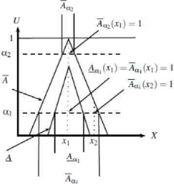
α − cuts of IVFS 14
According to the possibility and nessesity models of tanaka, the type-1 fuzzy regression model can be rewiten as:
The objective function is the sum of squared spreads of the upper and lower estimations.
The type-1 fuzzy regression problem can be reduced to the following two quadratic programming (QP)2,20. H is chosen as the degree of the fitting of the fuzzy linear model by the decision-maker.
Possibility model:
Necessity model:
3. Proposed type-2 fuzzy regression
Type-1 FLSs cannot fully handle high levels of uncertainties existing in most of the real world applications. The reason lies behind the fact that type-1 FLSs employs crisp and “precise” type-1 fuzzy sets. A type-2 FLS can handle higher uncertainty levels to produce improved performance. Type-2 FLSs have a variety of real world applications, in business and finance domains, in electrical energy domain, real-world automatic control, healthcare and medical domains 21–24. The membership functions of type-2 fuzzy sets are three dimensional and include a footprint of uncertainty. It is the third dimension of type-2 fuzzy sets, i.e. the footprint of uncertainty that additional degrees of freedom are provided, which in turn makes it possible to model and handle uncertainties 25.
Interval type-2 fuzzy sets are the most widely used type-2 fuzzy sets, since on the one hand they are simple to use and, on the other hand it is very difficult to justify the use of any kind of type-2 fuzzy set. In this case, the membership function is an interval type-2 fuzzy set which can be represented only by its FOU.
In this section, at first, proposed interval type-2 fuzzy regression model was formulated. Thereafter, this model developed to piecewise type-2 fuzzy regression and multivariate model.
Concerning Arianna Mencattini et al. 26, we will denote this kind of type-2 interval as Ãj = [[auj alj], bj, [clj cuj]] such that LMFÃ = (alj, bj, clj), UMFÃ = (auj, bj, cuj) and auj ≤ alj ≤ bj ≤ clj ≤ auj.
The observed output data is the interval type-2 fuzzy number ỹi = ([piu pil], qi, [ril riu]).
3.1. Proposed linear interval type-2 fuzzy regression
Since an IT2FS can be completely determined using its FOU and FOU is bounded by two membership functions LMF and UMF (I.e.by two type-1 MFs), this model has been built based on the possibility model for UMF and the necessity model for LMF. These two models, besides minimization the vagueness in secondary membership function, help to find an appropriate fit for the predicted value into the observed value.
To formulate a fuzzy linear regression model, the followings are assumed to hold.
- 1.
The data can be represented by an interval type-2 fuzzy linear model,
where Ỹi and Ãj are perfectly normal IT2FS and xj is positive.According to the model, the supports of LMF and UMF were obtained as the following:
Thus: - 2.
The degree of the fitting of the estimated value
In fact, the fundamental idea is to obtain parameters auj, alj, bj, clj, cuj of coefficient Ãj such that:
It means that the possibility model for UMFs and the necessity model for LMFs are used respectively. Because it is enough to close the membership functions of the observed and predicted values as much as possible and an h-cut of the observed value is included in the predicted value (Fig. 2). - 3.
The objective function is defined by J = J1 + J2 – J3 + J4.
That minimizing of J1 minimizes the vagueness of secondary membership function; and J2 minimizes the vagueness of LMF of Ỹ that is a type-1 fuzzy set. J4 minimizes the distance point with the highest membership value in a fuzzy estimated response and the point with the highest membership value in the corresponding observed response. But J3 is used for the necessity problem, and hence it should be maximized.
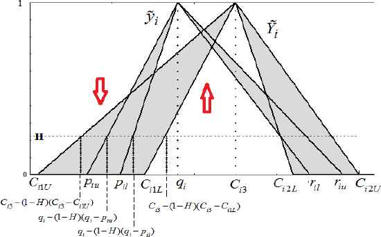
Degree of fitting of Ỹ to ỹ
More specially, our problem is to find out the fuzzy parameters auj, alj, bj, clj, cuj, which are the solution of the following two QP problems besides two extra objective functions (Fig.2):
QP problem of (11) and (12) are possibility and necessity model that used for UMF and LMF respectively.
More specifically, we can rewrite our problem as following:
3.2. Piecewise type-2 fuzzy regression
Linear models are inadequate in handling fluctuating data. Therefore, it is necessary for the model to be developed to the piecewise model. One of the advantages of our proposed model is that it can be easily extended to the piecewise model. Two QP formulations are presented to determine the necessity area for LMF and the possibility area for UMF by the interval type-2 fuzzy piecewise regression model.
The data can be represented by a piecewise interval type-2 fuzzy linear model:
P = {P1, P2, …, Pk} are the values of variable x subject to an ordering constraint P1 < P2 < … < Pk, k ≤ n. The practitioner can specify the number and position of change-points according to the data distribution.
In this model only calculation of Ci1U, Ci1L, Ci3, Ci2L, Ci2U are different from Linear model.
Preposition: If
3.3. Multivariate piecewise type-2 fuzzy regression
In many applications, there is more than one input, In this regard, to be able to deal with the problem of multiple inputs; multivariate model was required to be formulated.
Multivariate case can be viewed as a straightforward generalization of the previous case so that the used concepts are the same.
The output may be generally related to the q input. Every input could have some change -point. The multivariate model is as follow:
4. Numerical results
To evaluate the performance of the proposed model, a hybrid standard error of estimates (HS), standard deviation (Sỹ), hybrid correlation coefficient (HR), root mean square error (RMSE), and R- squared (R2) were used and defined as follows16,17:
4.1. Example 1
We have used the data of example 1 given in Hosseinzadeh et al. paper to evaluate the ability of our model. The interval type-2 fuzzy regression model is Ỹi = Ã0 + Ã0xi, where Ã0 = ([1.5 5.3], 5.52, [5.7 9.06]), Ã1 = ([0.6 1.05], 1.27, [1.49 2.02]).
The Piecewise interval type-2 fuzzy regression model is as follow:
The results of the two models are showed in Fig.3, Fig.4 (Continued) and table 1 (Continued). The proposed models are more efficient than the previous models, especially when the predicted values are defuzzyfied finally (the RMSE and R2 values show this claim). In our proposed piecewise model, in addition to the LMF and UMF of the predicted values, theirs FOU are included in the FOU of the observed values.
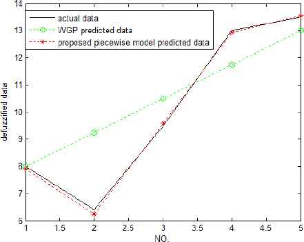
Defuzzyfied actual values, WGP predicted values and proposed T2FLR model predicted values
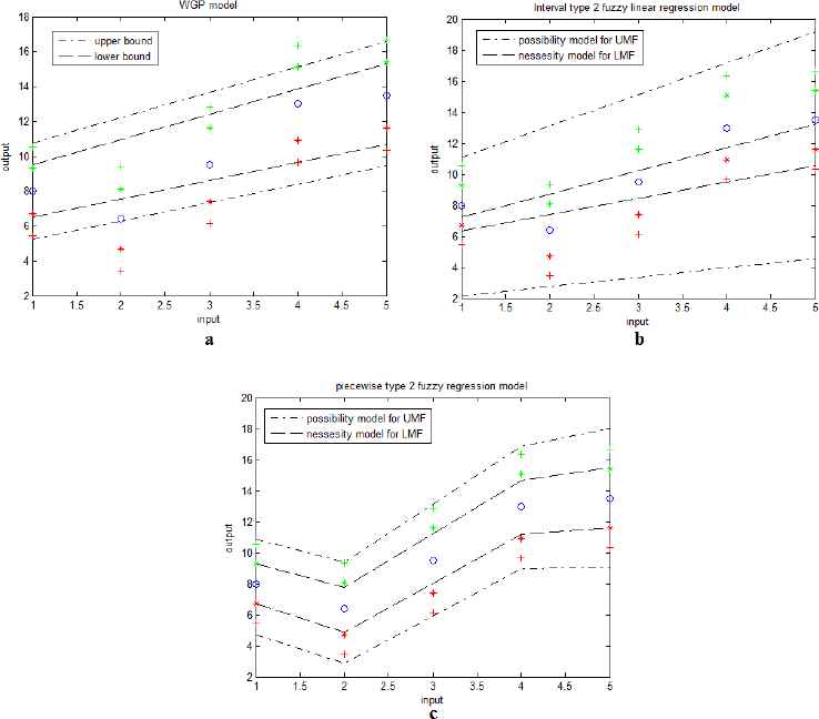
a) WGP model 17. b) Proposed interval T2FLR model. c) Proposed T2FLR model
4.2. Example 2
We use example 2 of Hosseinzadeh et al. paper for a multivariate model. The proposed model obtain the relationship between sodium percentage SP, as a function of three soil variables including the percentage of organic matter content (OM), sand content (SAND) and SILT, as the independent variables 17. OM=2, SAND=24, SILT=41, 44 are chosen as change-point, then:
As Fig.5 and table 2 (Continued) shows, RMSE, HS and Sỹ of proposed model with IT2FS coefficients is less than those of Poleshchuk et al.’s model and WGP model. In addition, the piecewise model has the maximum value of R2 and HR2 . These values in Table 2 show that, the predictive ability of our model is better than the predictive ability of earlier T2FS models.
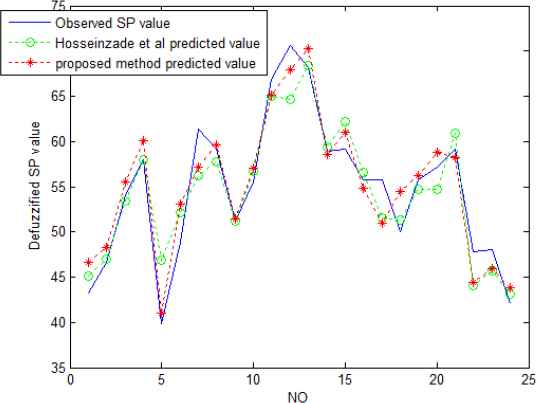
Defuzzified Observed values and predicted values in multivariate T2FLR
In multivariate model, HS of our model is greater than WGP model, because HS has been defined based on the distances of supports of membership function like WGP model, but our model is based on the possibility and necessity models. This doesn’t cause our research to be any less valuable. In fact, in most of the application, the results must be presented in a crisp form, which makes that RMSE comparison even more significant.
| HS | HR 2 | Sỹ | RMSE | R 2 | |
|---|---|---|---|---|---|
| Type-1 fuzzy regression 2 | 5.2 | 0.61 | 7.12 | 2.95 | 59.8% |
| Poleshchuk et al approach 16 | 3.77 | 0.68 | 6.20 | 1.82 | 66.2% |
| WGP approach 17 | 2.93 | 0.732 | 4.45 | 1.47 | 69.6% |
| Proposed Linear Type-2 fuzzy regression model | 4.01 | 0.758 | 4.51 | 1.2 | 71.1% |
| Proposed piecewise type-2 fuzzy regression model | 1.90 | 1.08 | 4.12 | 0.11 | 99.8 |
Comparing HS and RMSE in example 1
| HS | HR 2 | Sỹ | RMSE | R 2 | |
|---|---|---|---|---|---|
| Type-1 fuzzy regression 2 | 10.78 | 0.701 | 15.21 | 4.8 | 69.4% |
| Poleshchuk et al approach 16 | 7.19 | 0.758 | 14.45 | 3.7 | 78.3% |
| WGP approach 17 | 5.58 | 0.779 | 11.10 | 3.1 | 81.35% |
| Proposed Linear Type-2 fuzzy regression model | 9 | 0.766 | 10.98 | 2.6 | 83.51% |
| Proposed piecewise type-2 fuzzy regression model | 5.5 | 0.803 | 8.12 | 2.1 | 87.52% |
Comparing HS and RME in multivariate model
5. Conclusions
This study presents a type-2 fuzzy regression model according to the possibility and necessity model. In this model, vagueness is minimized, under the circumstances where the h-cut of observed value is included in predicted value. In this case, both observed values and predicted values are interval type-2 fuzzy numbers. In this model both primary and secondary membership function of predicted value fit the observed value. Developing model to piecewise model makes it helpful in dealing with the fluctuating data.
The numerical examples in this study are more accurate than the ones presented in the existing literature. According to the numerical examples, the matching of the predicted and the observed values is observed to have happened closer than the ones reported in the previous works. In most application, results should be reported in the crisp form and in proposed model the results are more accurate after the defuzzification, which is shown by RMSE.
Only one type of type-2 fuzzy sets is discussed here, but many types of type-2 fuzzy sets can be treated through developing same concept as in this paper. Yet, most of high vague phenomenon might be well identified by this model.
References
Cite this article
TY  - JOUR
AU  - Narges Shafaei Bajestani
AU  - Ali Vahidian Kamyad
AU  - Assef Zare
PY  - 2017
DA  - 2017/02/22
TI  - A Piecewise Type-2 Fuzzy Regression Model
JO  - International Journal of Computational Intelligence Systems
SP  - 734
EP  - 744
VL  - 10
IS  - 1
SN  - 1875-6883
UR  - https://doi.org/10.2991/ijcis.2017.10.1.49
DO  - 10.2991/ijcis.2017.10.1.49
ID  - Bajestani2017
ER  -