
Multi-Dimensional Indexing System Considering Distributions of Sub-indexes and Data
- DOI
- 10.2991/ijndc.k.191118.002How to use a DOI?
- Keywords
- Multi-dimensional index; parallel processing; retrieval performance; dissimilarity; distribution
- Abstract
This paper experimentally evaluates the parallel multi-dimensional indexing system indexing data by using several multi-dimensional indexes and retrieving required data from them in parallel. A constant number of data are indexed into a sub-index. The sub-index is inserted into an index in a computational node. After the number of sub-indexes in a computational node is evaluated, the area managed by each index is evaluated so that the numbers of sub-indexes become equal, and the data are widely distributed. It is experimentally shown that this method has good performance for skewed data.
- Copyright
- © 2019 The Authors. Published by Atlantis Press SARL.
- Open Access
- This is an open access article distributed under the CC BY-NC 4.0 license (http://creativecommons.org/licenses/by-nc/4.0/).
1. INTRODUCTION
The development of information technology and personal computers enable us to get various multimedia data. In order to retrieve these data quickly, it is necessary to construct a multi-dimensional index including the R-tree family [1–3]. However, when the index becomes large, insertion time and retrieval time become long. The previous researches of the parallel multi-dimensional index have tried to improve the retrieval performance, although these does not consider the insertion performance [3–7]. When we must store multimedia data continuously, it is required to construct a multi-dimensional index within a limited time.
Funaki et al. [8] have proposed the parallel multi-dimensional indexing system that constructs an index within a limited time and retrieves data quickly. This index system has three kinds of computing nodes: a Reception-Node (RN) for inserting data, a Normal-Node (NN) for storing data, and a Representative-Node (PN) for retrieving data. This index system also introduced three kinds of R-tree indexes: a Reception-Index (RI), a Whole-Index (WI), and a Partial-Index (PI). Data are indexed by an RI in the RN. After a certain number of data are indexed by an RI, it is moved to an NN and becomes a PI. A PI is managed by a WI in an NN. In the retrieval, a query is sent to a PN and is forwarded to the RN and all NNs. A PN is waiting for receiving results from the RN and the NNs. The indexing system mentioned above can quickly insert and retrieve a large number of multimedia data [9]. This parallel multi-dimensional indexing system was revised for improving the performance of insertion and retrieval [10]. For insertion, two RNs were introduced, and insertion was executed without a pause. An Administrative-Node (AN) was introduced in order to control these RNs. To reduce the retrieval time, PIs are distributed so that each NN has the almost same number of PIs as one another. The performance evaluation showed that the revised methods could improve the performances of insertion and retrieval.
The revised parallel multi-dimensional indexing system was evaluated by using skewed data and real data [11]. The experimental results revealed that the revised system still could not uniformly distribute PIs and that the retrieval performance degraded in some cases. Nakanishi et al. [12] proposed the methods of uniformly distributing PIs to NNs. In the previous system, the dissimilarity (distance) of the RI and a WI in an NN is firstly evaluated, and the numbers of PIs in NNs are secondarily evaluated before an RI is sent to an NN. The method proposed by Nakanishi et al. changes this order. This method firstly evaluates the numbers of PIs in NNs and then evaluates the dissimilarity. This could distribute PIs more uniformly than the previous method. This will result in the improvement of retrieval performance. The new dissimilarity calculation methods were also proposed [12]. These methods use PIs rather than the WI in calculating dissimilarity. This will be able to consider the distribution of PIs. This results in the precise decision of the NN to which the RI should be sent.
This paper experimentally shows that a combination of the evaluation method and a dissimilarity calculation method gives us good retrieval performance, especially for skewed data.
The remainder of this paper is structured as follows. Section 2 describes the parallel multi-dimensional indexing system [10]. Section 3 describes the revised parallel multi-dimensional indexing system [12]. Section 4 evaluates the revised system. Section 5 gives some considerations. Finally, Section 6 concludes this paper.
2. MULTI-DIMENSIONAL INDEXING SYSTEM
If data continue to be indexed by an index for a long time, the insertion time becomes long because of the decision of the insertion place and reorganization of the index structure. The parallel multi-dimensional indexing system that can insert and retrieve a large number of data quickly was proposed [8,9], and improved [10]. Figure 1 shows the organization of the parallel multi-dimensional indexing system [10].
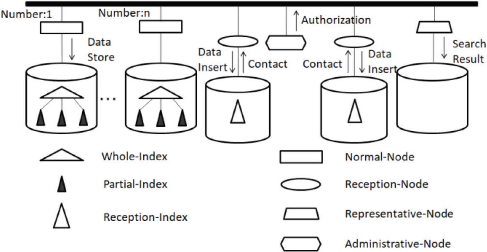
Parallel multi-dimensional indexing system.
This system has four kinds of computing nodes: an RN, an AN, an NN, and a PN. Each computing node has its own disk storage. All computing nodes are connected to one another through a bus.
2.1. Overview
An RN receives new data and indexes them by RI.
An AN manages various manipulation of insertion in two RNs. The AN confirms which RN indexes data and checks the remaining number of data that could be indexed by the RI.
Normal-nodes, each of which has a serial number, store data in the form of indexes. An NN has a WI and PIs. In a WI, a PI is managed as a rectangle, which is represented with a Minimum Bounding Rectangle (MBR) and is an entry of a node of the R-tree structure index.
A PN receives a query. As soon as a PN forward a query to all NNs and the RN, these nodes start to search data by using R-tree indexes. The retrieval results are sent back to the PN from the RN and all the NNs. The PN returns the retrieval result to the user.
2.2. Distribution Schemes
Data are indexed by an RI. When the RI grows to the predefined maximum size, the RI is moved to one of NNs. Here, it is important to select the destination node to which the RI is moved so that this selection can minimize the retrieval time. An RI is sent to the NN when the similarity is low, or the dissimilarity is high.
Three dissimilarity calculations are as follows:
- •
Area expansion: When an NN receives an RI, the NN calculates an expanded MBR area. The expanded MBR area is used as dissimilarity. The RI is moved to the NN whose MBR’s area expansion is the maximum one.
- •
Overlap: The area overlapped between the MBR of a WI of an NN and the MBR of the RI of the RN is used as the similarity. The RI is sent to the NN whose overlapped area between the two MBRs is the smallest one.
- •
Proximity: Proximity [4] of two MBRs is calculated by considering the degree of the overlap or distance of the MBRs. The formula for overlap MBRs is different from that for non-overlap MBRs [4]. The proximity of two MBRs is used as a similarity. Each NN calculates proximity between the own MBR of the WI and the MBR of the RI. The RI is moved to the NN whose MBR of the WI has low proximity with the RI.
Kamel and Faloutsos [4] showed that the Proximity index was the most successful heuristics among several distribution schemes.
2.3. Methods for Balancing the Number of Partial-indexes
In order to obtain good performance, RIs must be distributed to all NNs equally.
Three methods for distributing RIs to all NNs equally were proposed. These methods are as follows [10]:
- •
Method (a): When all dissimilarity values are the same, the RI is sent to the NN having the least PIs. If not all of the dissimilarity values but some dissimilarity values are the same, the RI is sent to the NN having the least PIs.
- •
Method (b): When some dissimilarity values of NNs are the same, the RN checks other dissimilarity values and determines the destination of the RI. If a certain dissimilarity value is larger than the others, the RI is sent to the NN having the largest dissimilarity value. Otherwise, if some dissimilarity values, which are the same, are larger than the other, the RI is sent to the NN having the least PIs regardless of the dissimilarity values.
- •
Method (c): When some dissimilarity values are the same, the RI is sent to the NN having the least PIs, regardless of other dissimilarity values.
When all NNs have the same dissimilarity value and store the same number of PIs, the destination of the RI is the NN firstly created.
3. MULTI-DIMENSIONAL INDEXING SYSTEM REVISED
3.1. The Decision before Dissimilarity Calculation
The system described in Section 2 tries to select the destination NN based on the dissimilarity value in order to balance the number of PIs among NNs. However, depending on the dissimilarity values, only a part of NNs may be selected as the destination candidates. In this case, some NNs have more PIs than others. All of NNs could not have the same number of PIs.
To address this issue, Nakanishi et al. [12] proposed a method considering the number of PIs earlier than considering the dissimilarity. The steps of the proposed method are as follows:
- •
Step 1: Find the NN which has the least PIs before calculating the dissimilarity.
- •
Step 2: If only one NN can be found, the RI is sent to the NN.
- •
Step 3: Otherwise, the dissimilarities are calculated for the NNs found.
- •
Step 4: If one NN has the maximum dissimilarity, the RI is sent to the NN.
- •
Step 5: Otherwise, the RI is sent to the NN having the smallest serial number of the NN.
This method gives priority for NNs to have the same number of PIs. This method is called the Decision before Dissimilarity Calculation (DBDC) method. The method described in Section 2 decides the destination NN after the calculation of dissimilarity. This method is called the Decision after Dissimilarity Calculation (DADC) method.
3.2. Dissimilarity Calculation Methods
In order to prevent an RI from being sent to the NN having many PIs, additional three dissimilarity calculation methods were proposed [12].
3.2.1. Mean distance
The mean of the distances between the center of the MBR of the RI, which will be sent from an RN to an NN, and the centers of MBRs of PIs in an NN is adopted as dissimilarity. It is considered that the larger the mean distance is, the more the MBRs are apart. When an NN has many PIs, and some of them are close to the RI, the distance may be small. This may prevent such an NN from being selected as the destination candidate. This may result in the selection of an NN having a few PIs.
3.2.2. Proximity and the mean distance
Proximity has good performance for the dissimilarity [10,11]. Proximity and the mean distance are used in calculating dissimilarity. When two or more NNs have the same smallest proximity, the mean distance method is applied to only these NNs.
3.2.3. Proximity and the shortest distance
The shortest distance is used instead of the mean distance in the method described in Section 3.2.2. That is, the shortest distance between the center of the MBR of the RI and the centers of MBRs of the PIs in an NN is used as the dissimilarity. The shortest distances are calculated for the NNs having the same smallest proximity.
4. EVALUATION
We evaluate the methods described in Section 3 by using synthetic data and real data on a real machine.
4.1. Data Used
We use the following data sets.
- (i)
Synthetic data: We use uniformly distributed and skewed data as synthetic data. These are two-dimensional points. The number of data is 500,000, and 80 PIs are created for each kind of data.
- (a)
Uniformly distributed data: 500,000 points were randomly created. The range of coordinates of points is from zero to 232 − 1.
- (b)
Skewed data: We created 20 PIs, whose range of coordinates of points is from 0 and (232 − 1)/2. The points in these PIs follow the normal distribution with mean (232 − 1)/4 and variance (232 − 1)/20. We also created 60 PIs, whose range of coordinates of points was from (232 − 1)/2 and 232 − 1. The points in these PIs follow the normal distribution with mean (232 − 1) * 3/4 and variance (232 − 1)/20.
- (a)
- (ii)
Real data: We use block-level location reference information distributed from the location reference information download service of the Ministry of Land, Infrastructure, Transport, and Tourism, Japan [13]. Three values of the block identifier, the latitude, and the longitude are selected and used. We use the data of Nagano, Hokkaido, and Kyoto prefectures of the fiscal year 2018. The total number of data used is 1,072,619.
4.2. Experimental Environment
Experimental environment is as follows:
- •
CPU: Intel Xeon(R) CPU E5-2630 v4 @ 2.20 GHz x 2.
- •
Memory: 32 GB.
- •
Hard Disk Drive (HDD): SATAIII 500 GB.
- •
Flash Memory: BUFFALO RUF3-HKS32G-TS 32 GB.
- •
OS: Ubuntu 16.04LTS.
- •
Compiler: GCC version 5.3.1.
- •
Library of R tree: libspatialindex version 1.8.5-3 [14].
The HDD is for RNs, while the flash memory is assigned to an NN.
4.3. Experimental Method
The DBDC method is compared with the DADC method by using the insertion time, the retrieval time, and the distribution of the numbers of PIs.
Insertion is conducted five times for four, eight, and 16 NNs.
The following retrievals are conducted by varying the number of NNs as four, eight, and 16:
- (i)
Uniformly distributed data: The range queries, whose range is one-tenth of the whole range, are conducted.
- (ii)
Skewed data: Twenty PIs, whose range of coordinates of points was from zero to (232 – 1)/2, are retrieved.
- (iii)
Real data: The range queries, whose range is one-tenth of the whole range, to the data of Kyoto prefecture are conducted.
In the comparison, Method (b) of the DADC method is used because this method attained the best performance [11]. Every retrieval is conducted 10 times.
4.4. Experimental Results
In the figures showing the experimental results, the dissimilarity calculation method based on area expansion (overlap, proximity, mean distance, proximity and the mean distance, and proximity and the shortest distance, respectively) is abbreviated as “AE” (“OL,” “PR,” “DI,” “DA,” and “MD”). The round-robin method, where a PI is moved to an NN in a round-robin manner, is added and abbreviated as “RR.”
4.4.1. Uniformly distributed data
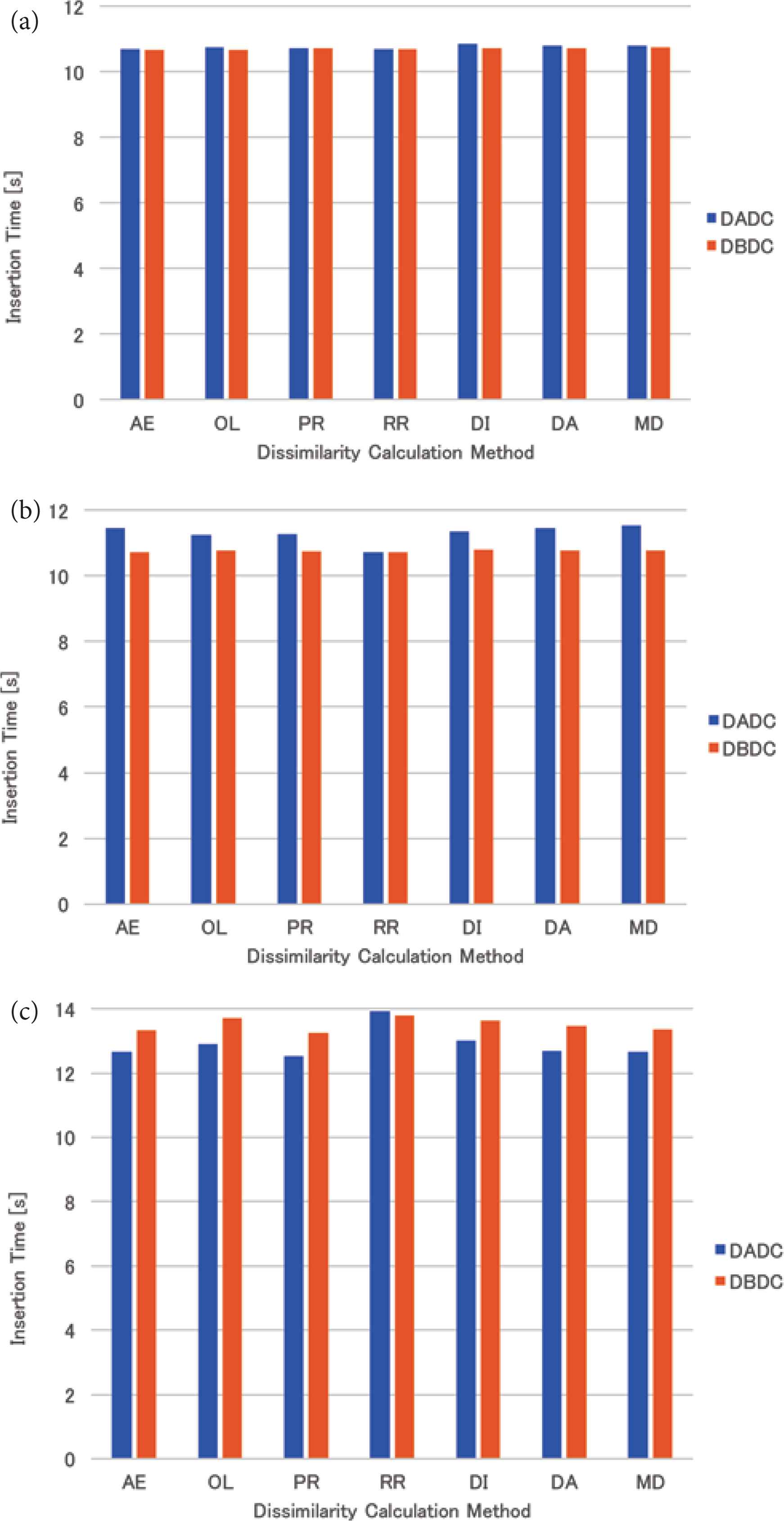
The mean insertion time of the uniformly distributed data for four (eight and 16, respectively) NNs is shown in Figure 2a–c. For four NNs, the insertion times of both methods were almost the same. For eight NNs, the insertion time of the DBDC method was slightly shorter than that of the DADC method, while the insertion time of the DBDC method was longer than that of the DADC method for 16 NNs. The insertion time for 16 NNs was longer than those for four and eight NNs.
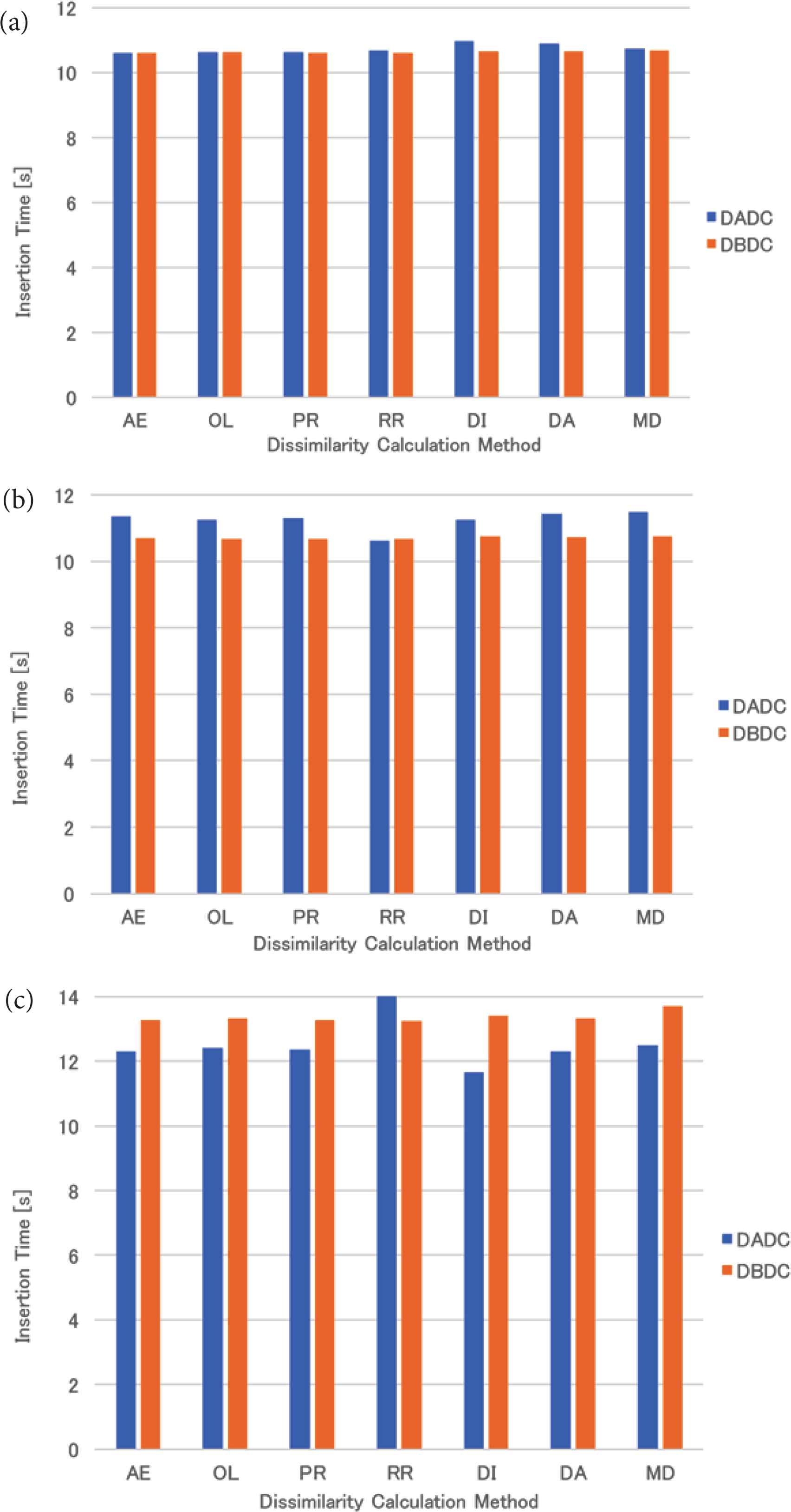
Insertion time of uniformly distributed data: (a) 4 NNs, (b) 8 NNs, (c) 16 NNs.
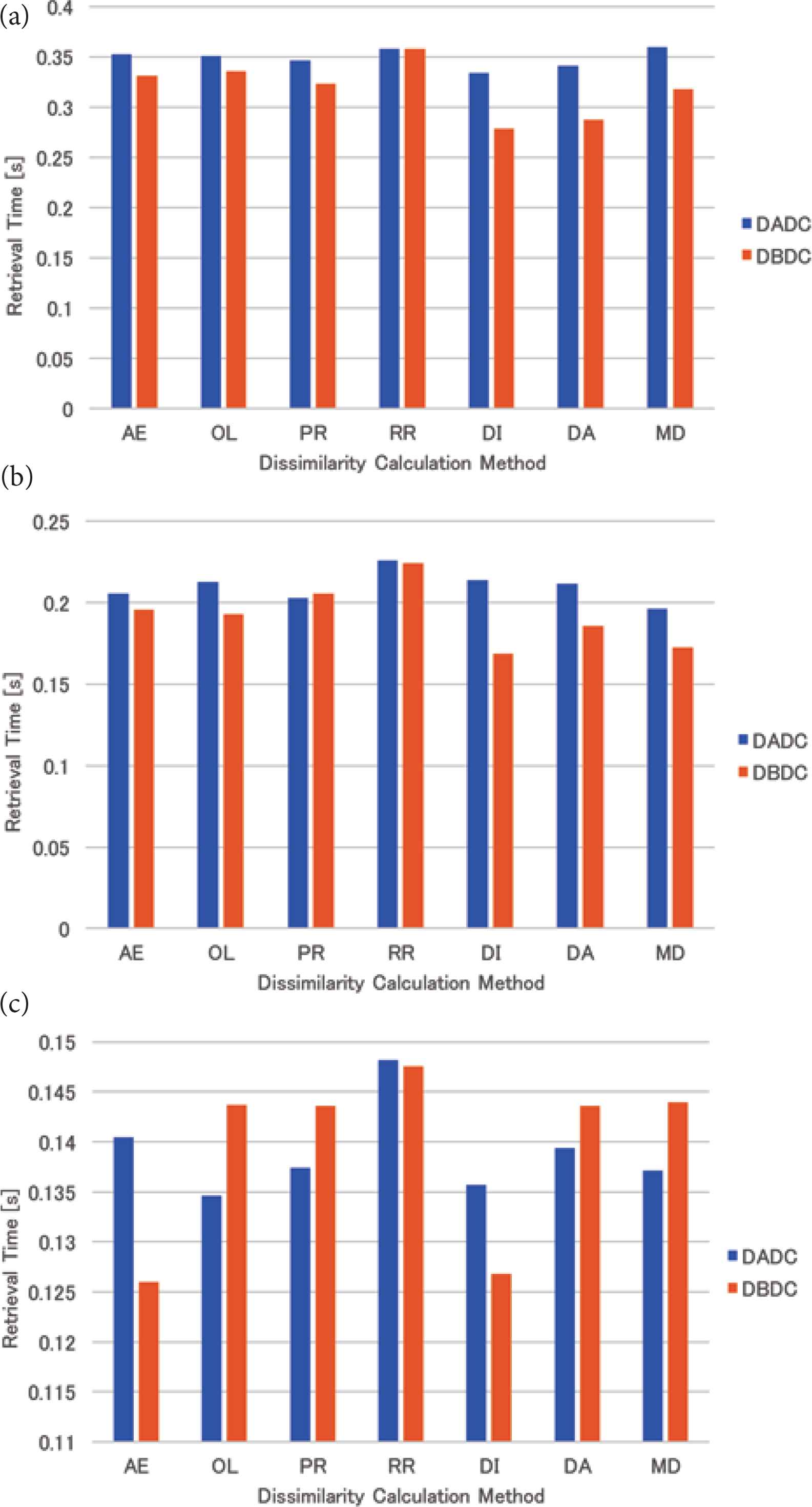
The mean retrieval time of the uniformly distributed data for four (eight and 16, respectively) NNs is shown in Figure 3a–c. The retrieval times of the DBDC method were the same regardless of the dissimilarity calculation methods and were shorter than those of the DADC method. Those of the DADC method with the methods based on the mean or shortest distance method (DI, DA, and MD) were worse than those of the DADC method with the other dissimilarity calculation methods for each number of NNs.
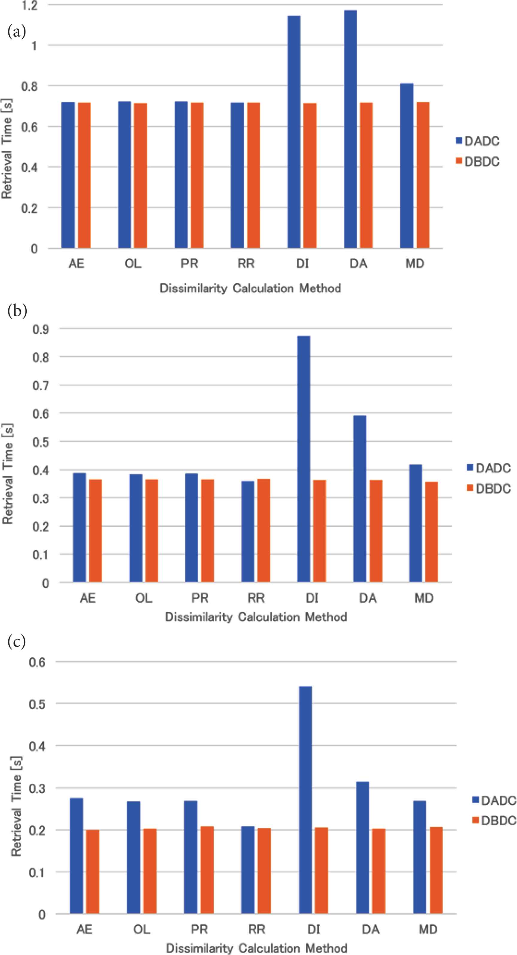
Retrieval time of uniformly distributed data: (a) 4 NNs, (b) 8 NNs, (c) 16 NNs.
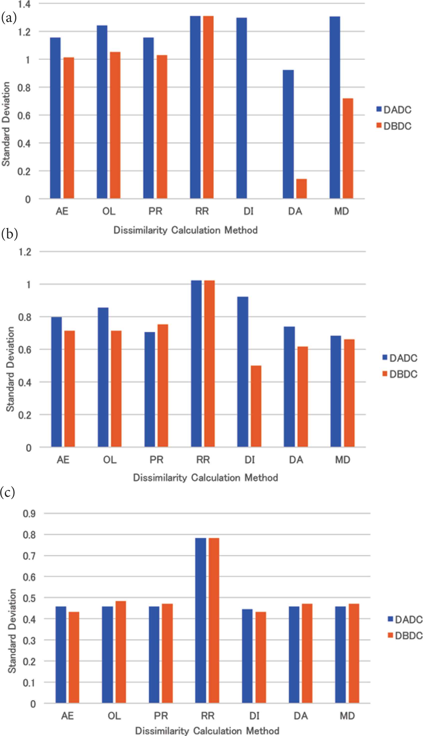
The mean standard deviation of the numbers of PIs in NNs for four (eight and 16, respectively) NNs is shown in Figure 4a–c. The standard deviation of the numbers of PIs in NNs was 0.0 for all dissimilarity calculation methods under the DBDC method, while that was larger than 0.0 for all dissimilarity calculation methods except for the RR method under the DADC method.
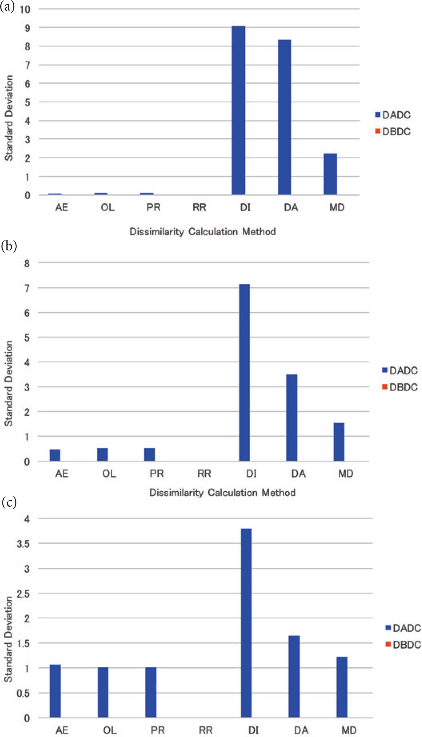
The standard deviation of the numbers of PIs in NNs for uniformly distributed data: (a) 4 NNs, (b) 8 NNs, (c) 16 NNs.
4.4.2. Skewed data
The mean insertion time of the skewed data for four (eight and 16, respectively) NNs is shown in Figure 5a–c. The tendency is the same as that of the uniformly distributed data as described in Section 4.4.1.
Insertion time of skewed data: (a) 4 NNs, (b) 8 NNs, (c) 16 NNs.
The mean retrieval time of the skewed data for four (eight and 16, respectively) NNs is shown in Figure 6a–c. For four (eight, respectively) NNs, the retrieval times of the DBDC method were shorter than those of the DADC method except for the round-robin (proximity) method. For 16 NNs, the DBDC method with the area expansion and the mean distance methods attained the best performance, while the performances of the DBDC method with the other dissimilarity calculation methods were worse than that of the DADC method except for the round-robin method.
Retrieval time of skewed data: (a) 4 NNs, (b) 8 NNs, (c) 16 NNs.
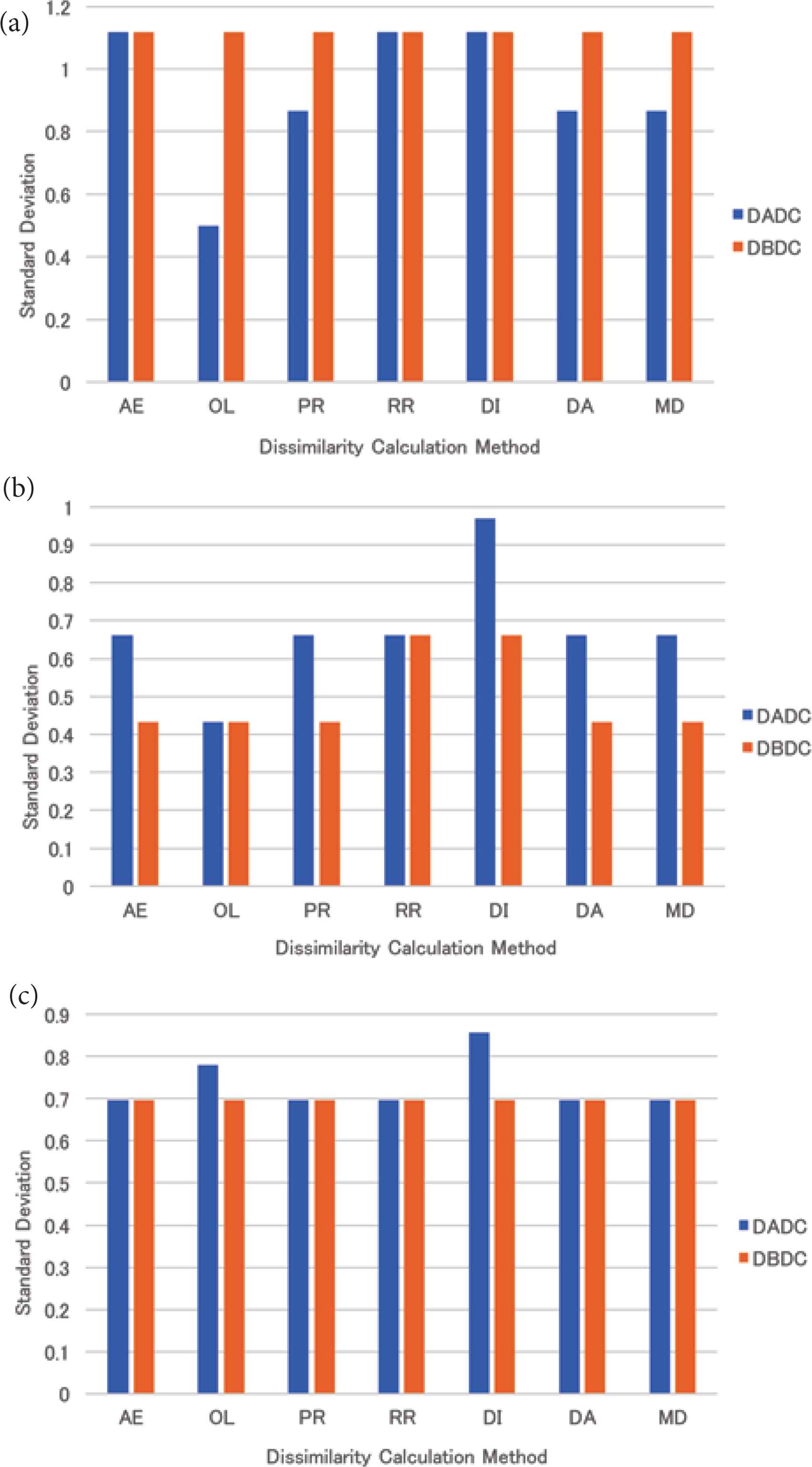
The mean standard deviation of the numbers of PIs accessed in the retrieval for four (eight and 16, respectively) NNs is shown in Figure 7a–c. The standard deviations of almost all dissimilarity methods were less than that of the RR method for four, eight, and 16 NNs. Those of the DBDC method were less than those of the DADC method for four and eight NNs. For 16 ones, those of the DADC and the DBDC methods were almost the same.
The standard deviation of the numbers of PIs accessed in retrieval for skewed data: (a) 4 NNs, (b) 8 NNs, (c) 16 NNs.
4.4.3. Real data
The mean insertion time of the real data for four (eight and 16, respectively) NNs is shown in Figure 8a–c. For four NNs, the insertion times of both methods were almost the same. For eight NNs, the insertion time of the DBDC method was slightly longer than that of the DADC method, while the insertion time of the DBDC method was shorter than that of the DADC method for 16 NNs. The tendency is opposite to that of the uniformly distributed data and that of the skewed data.

Insertion time of real data: (a) 4 NNs, (b) 8 NNs, (c) 16 NNs.
The mean retrieval time of the real data for four (eight and 16, respectively) NNs is shown in Figure 9a–c. For four NNs, the performance of the DBDC method only with the mean distance method was better than the DADC method. For the other dissimilarity calculation methods, the performance of the DBDC method was worse than the DADC method. For eight NNs, almost all the retrieval times of the DBDC methods were shorter than those of the DADC method. Those of the DBDC method with the overlap and the round-robin methods were worse than those of the DADC method. For 16 NNs, the retrieval times of the DADC and the DBDC methods were almost the same except for the DADC method with the mean distance method. As a result, the performance of the DBDC method with the mean distance method was better than that of the DADC method with it.
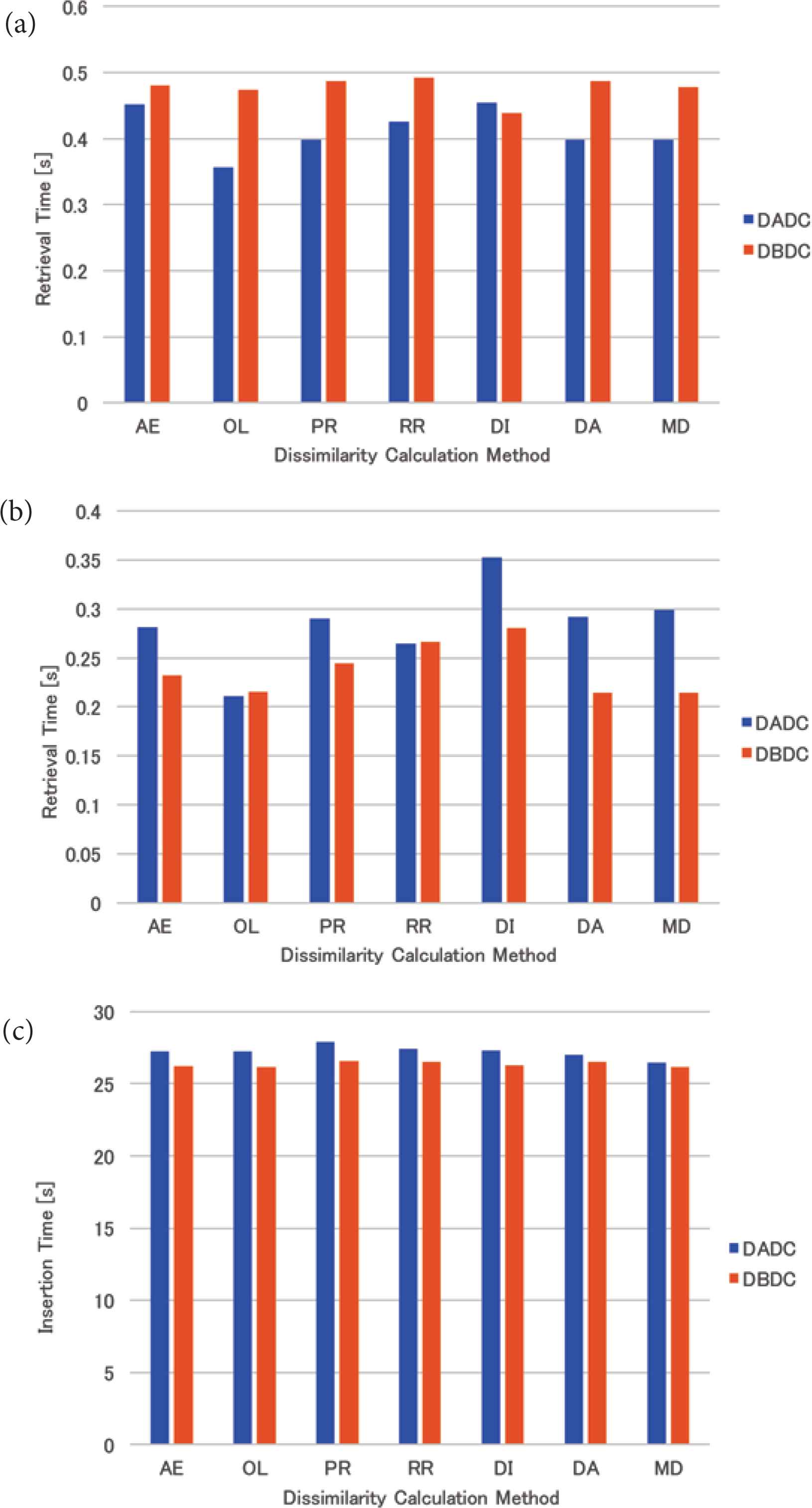
Retrieval time of real data: (a) 4 NNs, (b) 8 NNs, (c) 16 NNs.
The DBDC method could make the number of PIs in NNs the same, while the DADC method could not. The mean standard deviation of the numbers of PIs accessed in the retrieval for four (eight and 16, respectively) NNs is shown in Figure 10a–c. The numbers of PIs accessed in the retrieval were; however, not the same. The standard deviation of the numbers of PIs accessed in the retrieval under the DBDC method for four and 16 NNs was the same regardless of the dissimilarity calculation methods. The standard deviations were the same as that of the RR method. Under the DADC method, the standard deviations were smaller than or equal to that of the RR method for four NNs, while these were larger than or equal to that of the RR method for 16 NNs. For eight NNs, the DBDC method could make the standard deviation smaller than that of the RR method, while the DADC method could not.
The standard deviation of the numbers of PIs accessed in retrieval for real data: (a) 4 NNs, (b) 8 NNs, (c) 16 NNs.
5. CONSIDERATION
First, we give some considerations to the DADC and the DBDC methods. Next, we consider the dissimilarity calculation methods.
5.1. DADC and DBDC Methods
This paper evaluated the DBDC method, which restricts the target NNs according to the number of the PIs in them before calculating dissimilarity, so that NNs have the same number of PIs.
5.1.1. Insertion time
For four NNs, the insertion times of both the DBDC and the DADC methods were almost the same. For eight and 16 NNs, the insertion time of the DBDC method was slightly different from that of the DADC method. The insertion time of the DBDC method was not drastically different from that of the DADC method.
5.1.2. Retrieval time
For the uniformly distributed data, the retrieval time of the DBDC method was the same for all the dissimilarity calculation methods. It was the same as that based on the round-robin method. It is considered that PIs were distributed to NNs in the DBDC method just as in the RR method.
For the skewed data, the retrieval time of the DBDC method was shorter than that of the DADC method for four and eight NNs. For 16 NNs, the retrieval times of the DBDC method with the area expansion and the mean distance methods were shorter than those of the DADC method with them, while those of the DBDC method with the other dissimilarity calculation methods were longer than those of the DADC method with them. The DBDC method with the mean distance method had good performance regardless of the number of NNs. This method may distribute PIs to NNs by considering the distribution of data.
The retrieval times and the standard deviations of all dissimilarity calculation methods were smaller than those of the RR method for the skewed data for both the DADC and the DBDC methods as shown in Figures 6 and 7. As the RR method takes account of only the number of PIs, considering the dissimilarity is effective in treating skewed data for both the DBDC and the DADC methods.
For real data, the retrieval time of the DBDC method was worse than that of the DADC method for four NNs. This might be caused by that PIs were sent to an NN not as intended because the DBDC method restricts the target NN based on the number of PIs in an NN. On the other hand, the retrieval times of the DBDC method with five of seven dissimilarity calculation methods were better than those of the DADC method with them for eight NNs. For 16 NNs, the retrieval times of the DBDC method and the DADC method were almost the same except for that of the DADC method with the mean distance method. For eight and 16 NNs, the DBDC method sent PIs to NNs as intended. The retrieval time of the DBDC method with the mean distance method was always better than that of the DADC method with it. Under the DBDC method, the standard deviations of the numbers of PIs accessed in the retrieval were the same as that for the round-robin method for four and 16 NNs, while those were smaller than or equal to that for the round-robin method. This might result in good retrieval time at eight NNs.
5.2. Dissimilarity Calculation Methods
For the uniformly distributed data, the retrieval times of the DADC method with three dissimilarity calculation methods based on the mean or shortest distance method were bad, as shown in Figure 3. As the DADC method firstly calculates dissimilarity and selects the NN to which the RI is sent without any consideration of the number of PIs in an NN, some NNs have more PIs than others. This degrades the performance of the DADC method with them. These methods had better not be used with the DADC method.
For the skewed data, the mean or shortest distance-based methods with the DBDC method were better than the other methods with it for four and eight NNs. These distance-based methods worked well in the case that it decided an NN from those having the same number of PIs. For 16 NNs, the mean distance method with the DBDC method attained the best performance, while the other mean distance-based method and the shortest distance-based one with it failed.
6. CONCLUSION
This paper evaluated the DBDC method and the dissimilarity calculation methods based on the mean distance method to the parallel multi-dimensional indexing system. The DBDC method firstly considers the number of PIs and then calculates the dissimilarity. It was experimentally shown that this method with the mean distance method attained good retrieval performance compared with the DADC method and the DBDC method with the other dissimilarity calculation methods. It was also shown that considering dissimilarity is effective, especially for skewed data.
The mechanism of the DBDC and the DADC methods good for skewed data is not clear. Precise evaluation clarifying the mechanism good for skewed data is in future work. The AN has been introduced for controlling the RNs. This control may be undertaken by an RN. The evaluation of the architectures with and without the AN is also in future work. Concurrent insertion and retrieval of data are not supported yet. In order to support concurrent access of indexes, concurrency control of the index is required. The introduction of the concurrency control mechanism is in future work.
CONFLICTS OF INTEREST
The authors declare they have no conflicts of interest.
REFERENCES
Cite this article
TY  - JOUR
AU  - Kazuto Nakanishi
AU  - Teruhisa Hochin
AU  - Hiroki Nomiya
AU  - Hiroaki Hirata
PY  - 2019
DA  - 2019/12/06
TI  - Multi-Dimensional Indexing System Considering Distributions of Sub-indexes and Data
JO  - International Journal of Networked and Distributed Computing
SP  - 25
EP  - 33
VL  - 8
IS  - 1
SN  - 2211-7946
UR  - https://doi.org/10.2991/ijndc.k.191118.002
DO  - 10.2991/ijndc.k.191118.002
ID  - Nakanishi2019
ER  -