
Machine Learning in Failure Regions Detection and Parameters Analysis
- DOI
- 10.2991/ijndc.k.191204.001How to use a DOI?
- Keywords
- Testing; automation; machine learning; clustering; classification
- Abstract
Testing automation is one of the challenges facing the software development industry, especially for large complex products. This paper proposes a mechanism called Multi Stage Failure Detector (MSFD) for automating black box testing using different machine learning algorithms. The input to MSFD is the tool’s set of parameters and their value ranges. The parameter values are randomly sampled to produce a large number of parameter combinations that are fed into the software under test. Using neural networks, the resulting logs from the tool are classified into passing and failing logs and the failing logs are then clustered (using mean-shift clustering) into different failure types. MSFD provides visualization of the failures along with the responsible parameters. Experiments on and results for two real-world complex software products are provided, showing the ability of MSFD to detect all failures and cluster them into the correct failure types, thus reducing the analysis time of failures, improving coverage, and increasing productivity.
- Copyright
- © 2019 The Authors. Published by Atlantis Press SARL.
- Open Access
- This is an open access article distributed under the CC BY-NC 4.0 license (http://creativecommons.org/licenses/by-nc/4.0/).
1. INTRODUCTION
Testing has always been one of the hardest phases in software development life cycle, and increases in size and complexity of the software exponentially increase the number of failing regions and corner cases. Since testing consumes a huge portion of all development efforts, and requires even more effort for systems that require a high level of reliability, some kind of automation becomes a necessity. Different failures can have different execution traces, and to discover new unknown failures, or group different failure causes together, using traditional testing methods may no longer be feasible. The use of machine learning has been explored to solve various testing problems.
A category of machine learning research focuses on analyzing, prioritizing, and refining already existing test cases. In Briand et al. [1], the authors focused on refining the test suites by using a category partition method and trees to remove redundancies and discover uncovered parts with the test suite. In Lachmann [2], machine learning was applied to prioritize test cases by using some features within them (like test case age and number of defects) to prioritize and sort them. The problem of removing redundancy among test cases was addressed in Vangala et al. [3] by using unsupervised clustering to cluster similar test cases together. Also, reinforcement learning was used to select and prioritize the test cases [4].
Other research focuses on creating a test oracle. A deep learning model is built to act as the test oracle. The model is trained so that the output is similar to the Software under Test (SUT). The trained model is used to predict and detect any wrong output [5].
This paper proposes an automated approach using two cascaded machine learning algorithms, first to detect the failures in the software and then to cluster similar failures so the engineer would not have to inspect all executions of the software. The first problem is classification of the passing and failing executions, and for that, a shallow neural network is used. The second problem is clustering similar failures together, and for that, a mean-shift clustering is used. The rest of the paper is structured as follows. Related work is described in Section 2. Section 3 provides background on the different techniques used in this paper, including both text processing and machine learning algorithms. The proposed approach is described in Section 4. The experiments and results are discussed in Section 5. Conclusions are drawn in Section 6.
2. RELATED WORK
An important aspect of software testing is to detect unique failure regions in the software. The ability to detect these failure regions provides good testing coverage and avoids test case redundancy. Researchers have tackled this problem in different ways.
Random forests are used in Haran et al. [6] to detect whether or not there is a failure in the execution, according to the execution traces of the program, by using a small number of method counts as a feature set. This approach achieved an error rate of <7% when applied to all versions of a subject program for classifying failing and passing executions. Although it provided good results, it focused on the classification of passing and failing executions without any consideration of clustering the failures or identifying the unique failures.
In Dickinson et al. [7] and Podgurski et al. [8], clustering algorithms are used to cluster the execution profiles and detect different types of failures. The main drawback in these methods is that the number of clusters must be provided by the user i.e. the user must have insight into the number of failure types. In Dickinson et al. [7], the user must determine the optimum number of clusters, while in Podgurski et al. [8], the optimum number of clusters is not accurately determined, so a kind of visualization is provided to help determine the best clusters. In this work, the number of clusters is determined automatically by using methods explained in Section 4.
In Du et al. [9], a deep neural network model using Long- and Short-Term Memory (LSTM), is trained on the system logs to model the normal system behaviour. That is used to detect anomalies from the logs resulted from different tools which is similar to this work, and in Fu et al. [10] free text logs are changed into log keys and a finite state automation is trained on log sequences to present the normal work flow for each system component. At the same time, a performance measurement model is taught to detect the normal execution performance based on the log messages timing information. However an extra step is provided in this paper’s work which was not provided in Du et al. [9] and Fu et al. [10] that is after detecting these anomalies they are clustered into different failing regions.
3. BACKGROUND
The flow proposed in this work, detailed in Section 4, relies on text processing and machine learning algorithms. In this section, these technologies are discussed.
3.1. Term Frequency Inverse Document Frequency
Term frequency inverse document frequency (TF-IDF) [11] is an algorithm used to determine how important a word is to a document in a collection, or to the whole collection. TF-IDF determines the relative frequency of words in a specific document compared with the inverse proportion of that word over the entire document corpus. For example, if there is a corpus of documents and each set of these documents belongs to a certain category, to classify or cluster these documents, they first must be transformed into a bag-of-words [12]. The bag-of-words model is a type of representation of documents used in natural language processing, where the document is decomposed to a set of words, disregarding the grammar and word order. Each document in this corpus will have the same bag-of-words that was created from the whole corpus, but the values for each word in the bag-of-words for each document will be different. This value is calculated using the TF-IDF.
Given a document collection D, a word w, and an individual document d where d ∈ D, we calculate [Equation (1)]
3.2. Artificial Neural Networks
Artificial Neural Networks (ANNs) are designed to resemble the structure and information-processing capabilities of the brain [13]. The building blocks of this neural network are called neurons, where the network consists of one or more layers of these neurons. The interconnections between these neurons have certain variables, called weights. These weights store information during the training phase. The strength point of the neural networks is that it can extrapolate the learned information to produce or predict outputs that were not present in the training data (generalization). Neural networks are used to solve difficult and complex problems in many fields, like data mining, pattern recognition and functions approximation.
As shown in Figure 1, the neurons, which are the building blocks of the neural network, consist mainly of three elements. The first two are the weights (which are in the interconnections) and an adder or summation of the product of the input and the weights (which is called the net) with Equation (2)
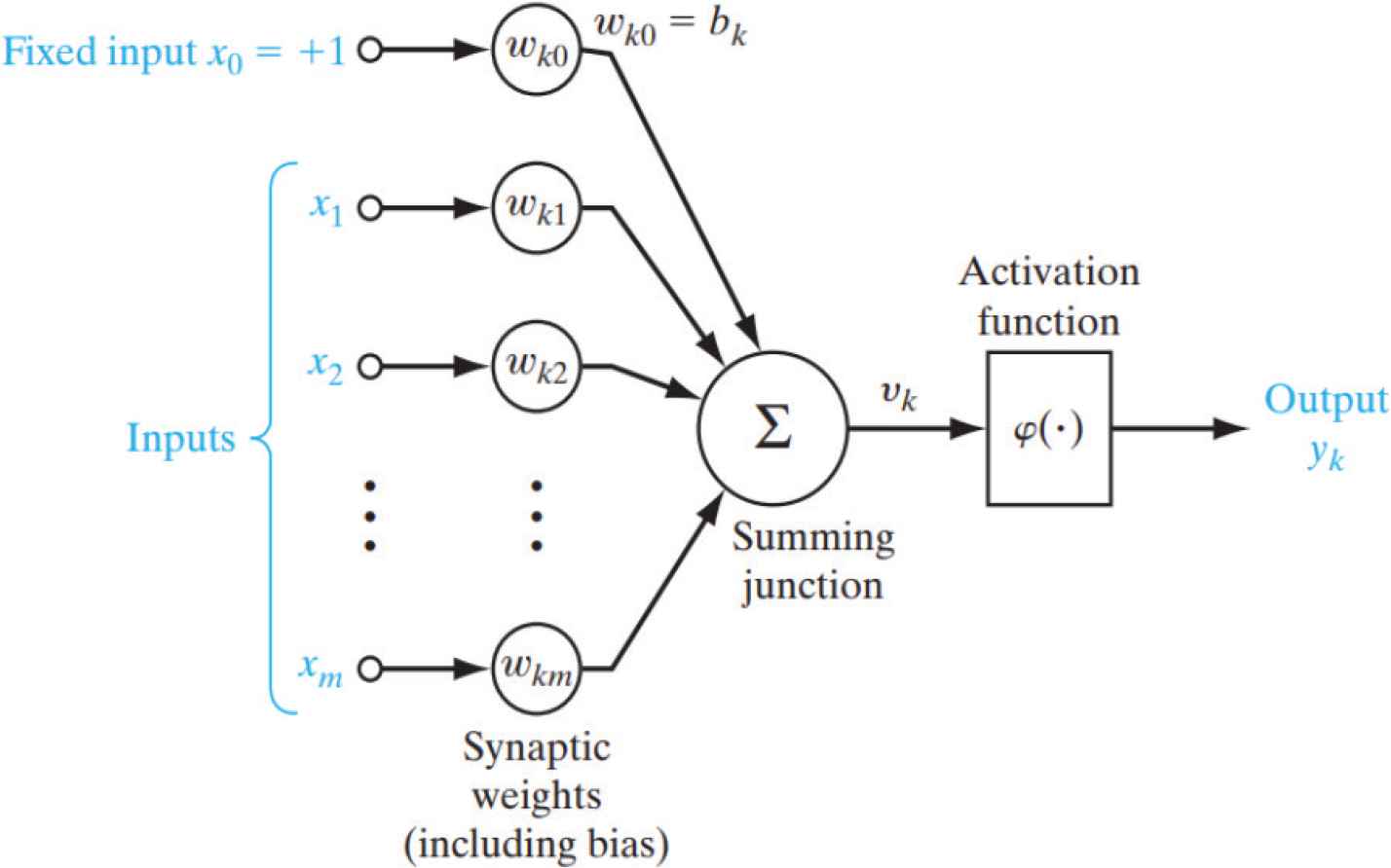
Structure of the neuron [11]
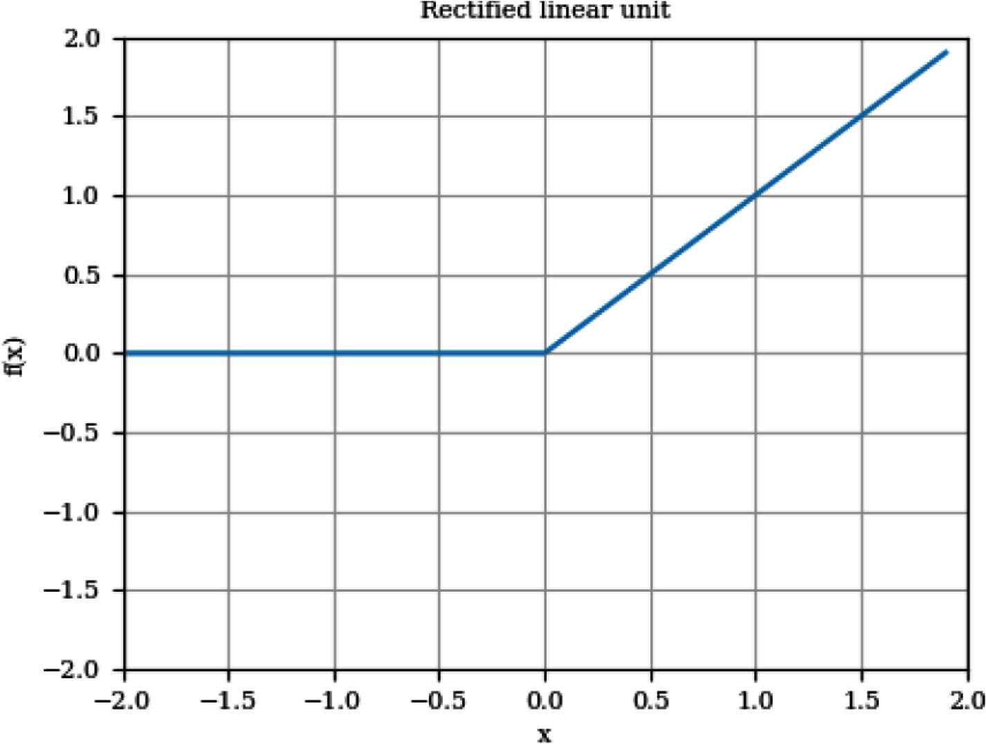
ReLU activation function
Another type of activation function is the softmax function [15]. The equation for this function is [Equation (4)]
This activation function enables the network to predict the probability that a certain input belongs to a certain class, instead of having an output of only 0 and 1.
3.3. Mean-shift Clustering
The mean shift algorithm was originally presented in 1975 by Fukunaga and Hostetler [16]. Mean shift is a hill-climbing algorithm that starts at a random point and keeps optimizing until reaching the optimum solution. Assume a set of points in a two-dimensional space. The kernel of the mean shift is a window with a center c, and radius (or bandwidth) r. Figure 3 shows the different steps for the algorithm. The first step (Figure 3a) is to choose a random point from the data points, which is selected as center to the kernel with a radius r. In the second step (Figure 3b), the mean of all points within the bandwidth is calculated according to the shape of the kernel. For example in a Gaussian kernel, each point has a certain weight that decreases exponentially by moving away from the center. In step three (Figure 3c), the calculated mean becomes the new center of the kernel, and a new mean is calculated. In step four (Figure 3d), when the calculated mean does not change after a number of iterations, then this cluster has reached convergence. Another point from the data set is chosen again, repeating steps 1 through 4. Although this algorithm seems simple, selecting the radius is a hard task, which is dependent on the data points provided.
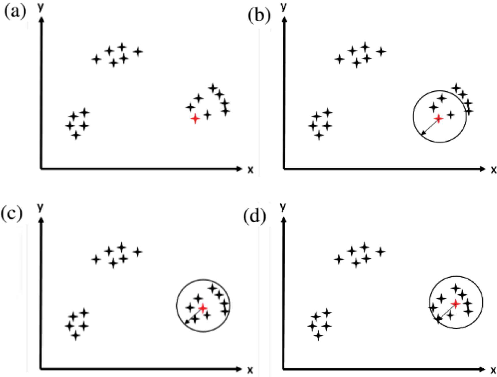
Mean-shift clustering algorithm. (a) Step 1. (b) Step 2. (c) Step 3. (d) Step 4
3.4. Singular Value Decomposition
Singular Value Decomposition (SVD) was developed by the differential geometers, but the first proof of SVD for rectangular and complex matrices was by Eckart and Young [17]. One of the applications of SVD is dimensionality reduction. In this section, a brief overview of the SVD will be provided. In the following Equation (5), a matrix A is decomposed into three matrices
4. METHODOLOGY
In this section, a detailed discussion of the proposed approach is provided. As shown in Figure 4, the Multi Stage Failure Detector (MSFD) consists mainly of two blocks; the first block is responsible for generating the test cases or the test scenarios, while the second block’s function is classifying the logs of the SUT and then clustering them to discover all the failing regions.
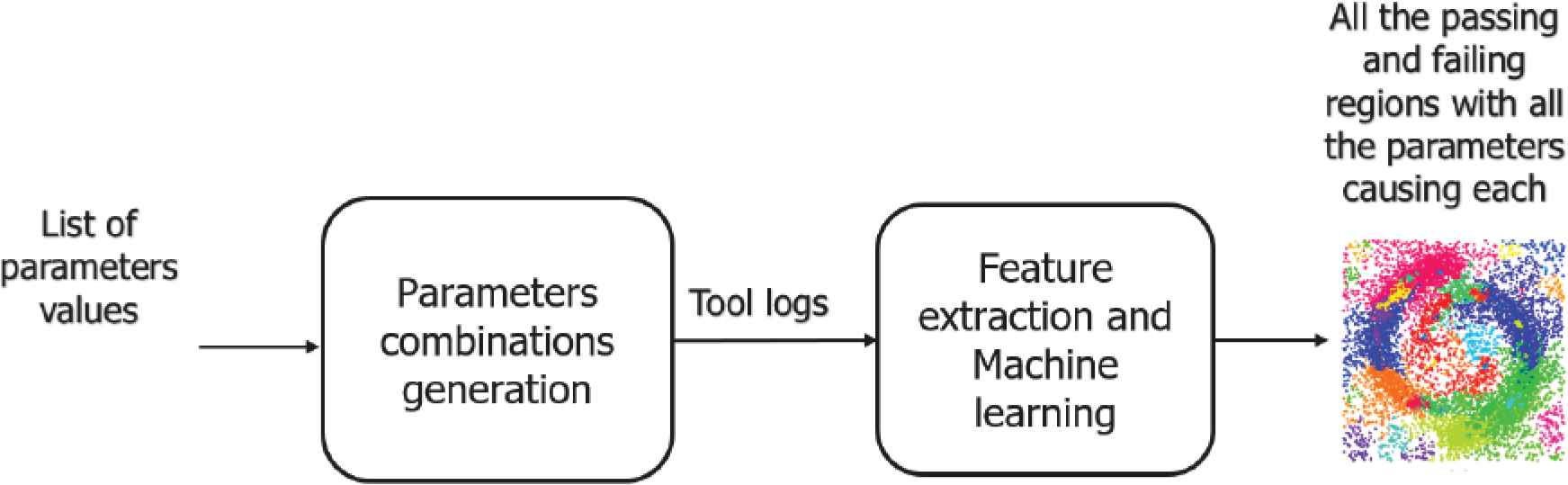
Multi stage failures detector main blocks
4.1. Parameters Combinations Generation
The input to MSFD are the parameters of the SUT and the ranges of values for these parameters. Random samples from all of these ranges are chosen, and all possible combinations for the selected samples are then executed. That is the MSFD uses the parameters combinations generated to run the SUT, which in return generates the logs that MSFD will use to determine the failing regions. After that, all the logs resulting from each execution are fed to the second block of the tool.
4.2. Feature Extraction and Machine Learning Models
As shown in Figure 5, the second block of MSFD consists mainly of three stages:
- (i)
Feature extraction.
- (ii)
Machine Learning: this stage is composed of two steps:
- •
Supervised learning using a feed-forward ANN for classification of logs into pass and fail logs
- •
Unsupervised learning using mean-shift clustering for clustering of failing logs
- •
- (iii)
Visualization of results.
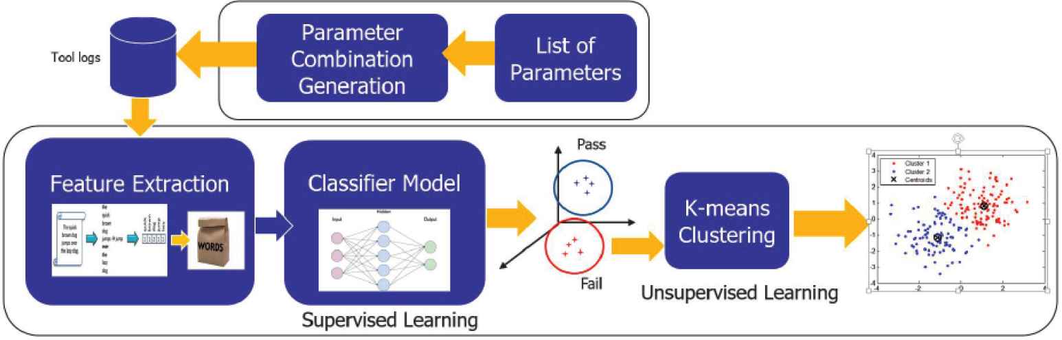
Multi stage failures detector detailed flow
4.2.1. Feature extraction
The generated logs are converted into a numerical representation using TF-IDF. The logs were first converted into a bag-of-words, and TF-IDF was then applied, transforming the logs into a vector of numerical values. Each value represents a score for the words of interest calculated using TF-IDF.
4.2.2. Machine learning
Classification of logs using ANN: A supervised machine learning model which is a fully connected feed-forward ANN, is used in this stage. The network consists of three layers: an input layer with a size equal to the feature vector, the hidden layer, which has a ReLU activation function and 32 nodes, and the last layer, which uses a softmax activation function to classify the passing and failing logs.
Unsupervised clustering using mean shift: The goal of this stage is to find the number of unique failures within the failing logs. Since this number is unknown, mean-shift clustering was used to cluster the failures. As discussed in the background section, the main drawback of this algorithm is selecting the ‘r’ or bandwidth value to determine the optimal number of clusters, so a solution had to be found to solve this issue. A solution for this problem was introduced in Pedregosa et al. [18] where the K-nearest neighbors algorithm was used. The number k is dependent upon the samples number and the k-NN algorithm was used to return the distances from a point to its neighbors. The max distance among these distances is selected for each point and the same procedure is repeated for all the points in the space. All these distances are then summed, and the average value calculated is the optimum bandwidth or radius to be used in the mean shift.
4.2.3. Visualization
Multi stage failure detector provides three types of visualizations:
- •
Failing logs visualizations: after the logs are transformed into numerical vectors using the TF-IDF and clustered, each of these numerical vectors’ dimensions is reduced to two dimensions using a truncated SVD (which is a version of the SVD mentioned in the background section), and implemented in Fukunaga and Hostetler [16] to be plotted. Such graphs help the user clearly see the failing logs, and how different they are from each other. Truncated SVD facilitates the viewing of the clusters of failures in two dimensions. The full information of the clusters and the associated log files is saved by the tool in a separate directory and can be examined by the user.
- •
Failing parameters visualizations: each cluster’s failing parameters are plotted, and if the number of parameters is more than two, truncated SVD is used to reduce their dimension to two dimensions.
- •
Parameters analysis visualizations: each parameter or a combination of two parameters is plotted to determine their accepted ranges of values.
4.3. Validation
The results of the MSFD were validated manually by examining each cluster, and examining the ranges resulted from the MSFD to make sure that the results are accurate.
5. EXPERIMENTS AND RESULTS
Multi stage failure detector was tested on two EDA tools which are Calibre® layout schema generator (LSG) tool and xCalibrate™ to evaluate its efficiency. In the following two sections, the results achieved from applying the MSFD on the two tools will be discussed.
5.1. Calibre® LSG
Calibre® LSG [19] is a tool for the random generation of realistic design-like layouts, without design rule violations. The tool uses a Monte Carlo method to apply randomness in the generation of layout clips by inserting basic unit patterns in a grid. These unit patterns represent simple rectangular and square polygons, as well as a unit pattern for inserting spaces in the design. Unit pattern sizes depend on the technology pitch value. During the generation of the layouts, known design rules are applied as constraints for unit pattern insertion. Once the rules are configured, an arbitrary size of layout clips can be generated.
The input to MFSD was the command that runs the LSG, along with 11 different parameters and the ranges to be tested for these parameters. The number of samples taken from each parameter range was set to be either three or two samples. That resulted in 20,736 combinations, which maps to the same number of logs. Since the tool to be tested produces a passing log only when all 11 parameters have a valid value (if there is even one parameter with an invalid value, the tool under test should produce an error message), the number of the passing logs is always much less than that of the failing logs.
5.1.1. Feature extraction
These logs were then fed to the feature extraction block shown in Figure 5, where the TF-IDF algorithm was applied to generate vectors of weights. After removing the stopping words (like a, the, an, is...), each of these logs was converted into a numeric vector of 64 rows (64 elements per vector). Each of these rows corresponds to a certain word. Examples of the captured words include “completed”, “count”, “cpu”, “creating”, “error”, “file”, “floating”, “successfully” and “zero”. Each of these words has a different score for each log’s vector. By examining this sample of words, it is clear that some weights are discriminating features for each of the passing and failing logs. Although some passing logs may contain the word “error”, and some failing logs may contain “successfully”, some combinations of word weights (like “error” with “completed”) may mean a passing run, while “successfully” with “zero” may be a failure.
5.1.2. Classification
The extracted features are used as input to the classification stage, which is the ANN. It was proven that providing a small training data set containing 1000 passing (positive) log samples and 1000 failing (negative) log samples, with 20% of them used as test data, and a shallow neural network as stated, was enough to draw the hyper-plane separating the passing logs and the failing logs, producing an accuracy of 100% on the test data. The result from this phase was classifying the 20,736 logs into 20,712 failing logs and 24 passing ones.
5.1.3. Clustering
The failing logs were then re-parsed, as TF-IDF was applied to them again, producing numerical vectors of 46 rows. Each of these rows again corresponds to a certain word. The TF-IDF was applied again because some of the words existed in the passing logs, but were not found in the failing ones, so the vectors of the failing logs had zero values for these words. Also, during the first TF-IDF representation, the weights of some specific words had larger values, since they were discriminating features for passing and failing logs, while in the case of being in a corpus containing only the failing logs, these words may have no real value. Reapplying the TF-IDF after the classification was for optimization (removing zeroes) and to achieve more accurate results. Examples of words captured in the second TF-IDF include “layer”, “margin”, “pattern col count”, “error”, “floating”, “id”, and “layer”. In the sample of captured words, the word ‘layer’ is captured two times. However, the first time, it is “layer” (with double quotes), while the second time, it is just layer. That happened because during the feature engineering phase, it was noticed that the error message that appeared was due to a failure caused by one of the parameters sometimes containing the name of that parameter within double quotes. As a result, a pattern separating normal words from double-quoted words was added to the TF-IDF allowing it to treat “layer” and layer as two different words with two different weights in the numerical vectors produced. Before adding the feature of separating quoted from unquoted keywords, some similar errors were grouped together, resulting in some of the clusters being combined with each other to produce a total of nine clusters, which is not the right number of clusters. After adding this feature, failing logs were clustered into 11 clusters, which is the right number of failure regions, producing a 100% accuracy result for the LSG.
5.1.4. Failure analysis
The third and last phase is the visualization phase, and as stated in the methodology section, MFSD provides three different visualizations: visualizing the logs, visualizing the failing parameters, and visualizing the ranges of acceptable parameter values discovered from running MFSD. The failing logs vectors contained 46 rows, which corresponds to 46 features and 46 dimensions. To visualize these results, a truncated version of the SVD was used to reduce the dimensions to two dimensions. The resulting graph is provided in Figure 6.
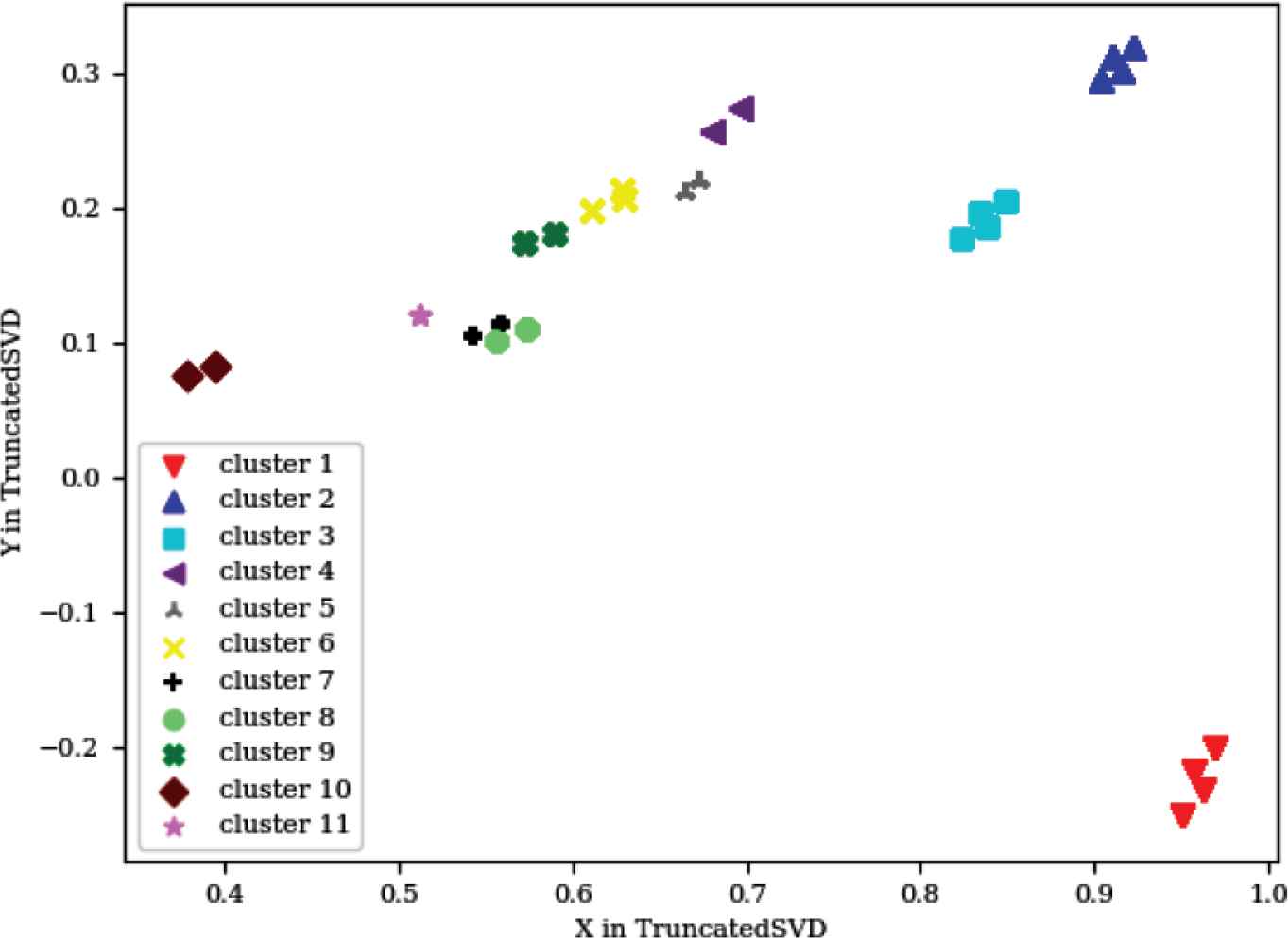
Layout schema generator failing logs
This graph represents 20,712 points, which corresponds to 20,712 failing logs clustered into 11 clusters. The number of points on this graph is much less than this number because logs resulting from similar failures were very close to each other in the high dimensional space. Upon decreasing the features into only two dimensions, these logs coincided. Some light green clusters (cluster 8 in Figure 6) also coincide with some black ones (cluster 7 in Figure 6), due to a small information loss resulting from the dimensionality reduction. All cluster information is saved in a directory by the tools and can be examined by the user. The second graph provided by this tool plots the parameters that caused each of these failures (Figure 7).
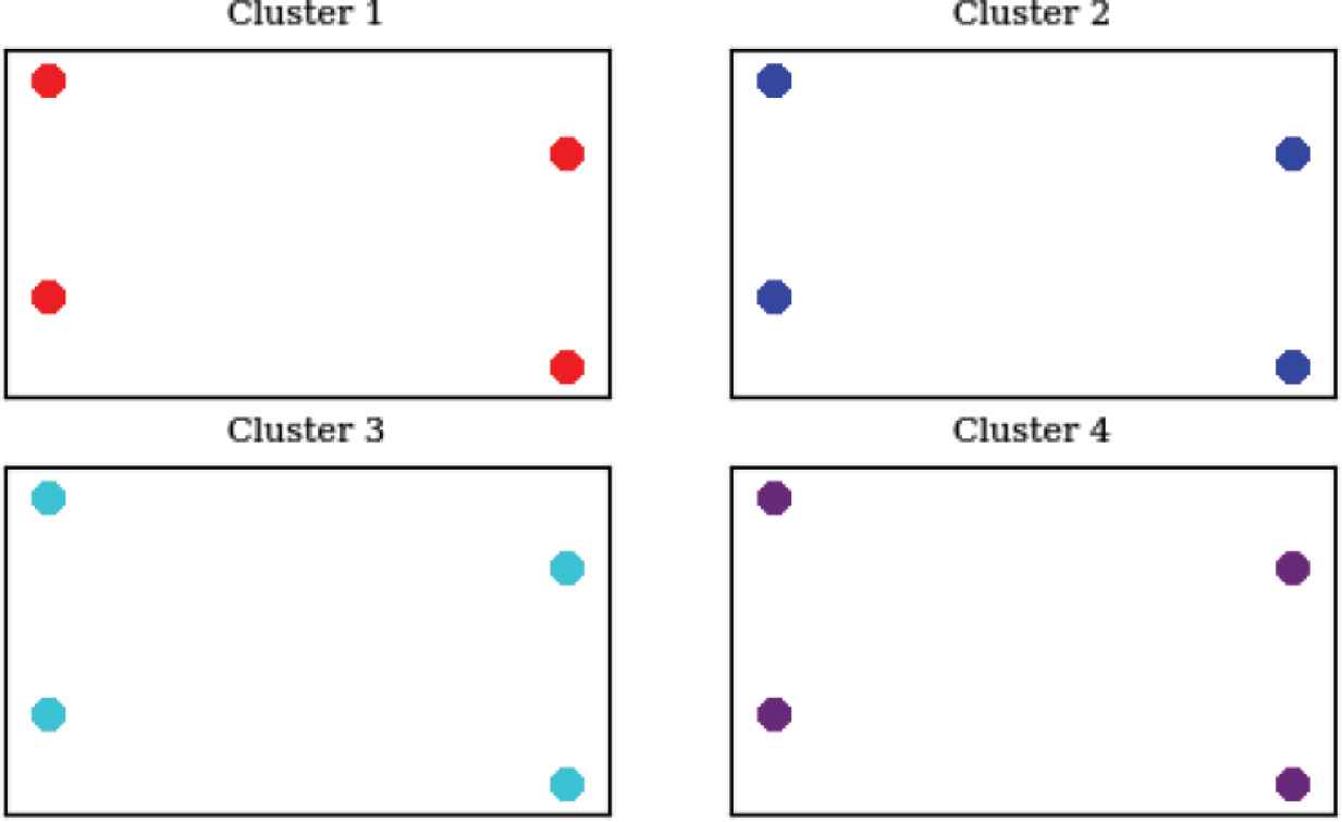
LSG failing clusters parameters
Each of the clusters shown in this graph contains a graphical representation of the 11 parameters that caused that error (only four clusters’ parameters are plotted here, but all 11 clusters can be plotted if needed). Since there are 11 parameters, a dimensionality reduction algorithm was applied and the truncated SVD was used again. So, if the user needed to analyze the set of parameters that caused the first kind of failure, taking four samples from cluster 1 is enough to cover cluster 1’s space, as shown in Figure 7. As demonstrated before, although the number of failure logs in cluster 1 is far more than four points, only four points are observed because they are close to each other in the higher dimension space (in this case, 11 dimensions), so they coincided in the lower one. The last graph provided by the MSFD is the representation of each parameter or combination of two parameters (Figure 8).
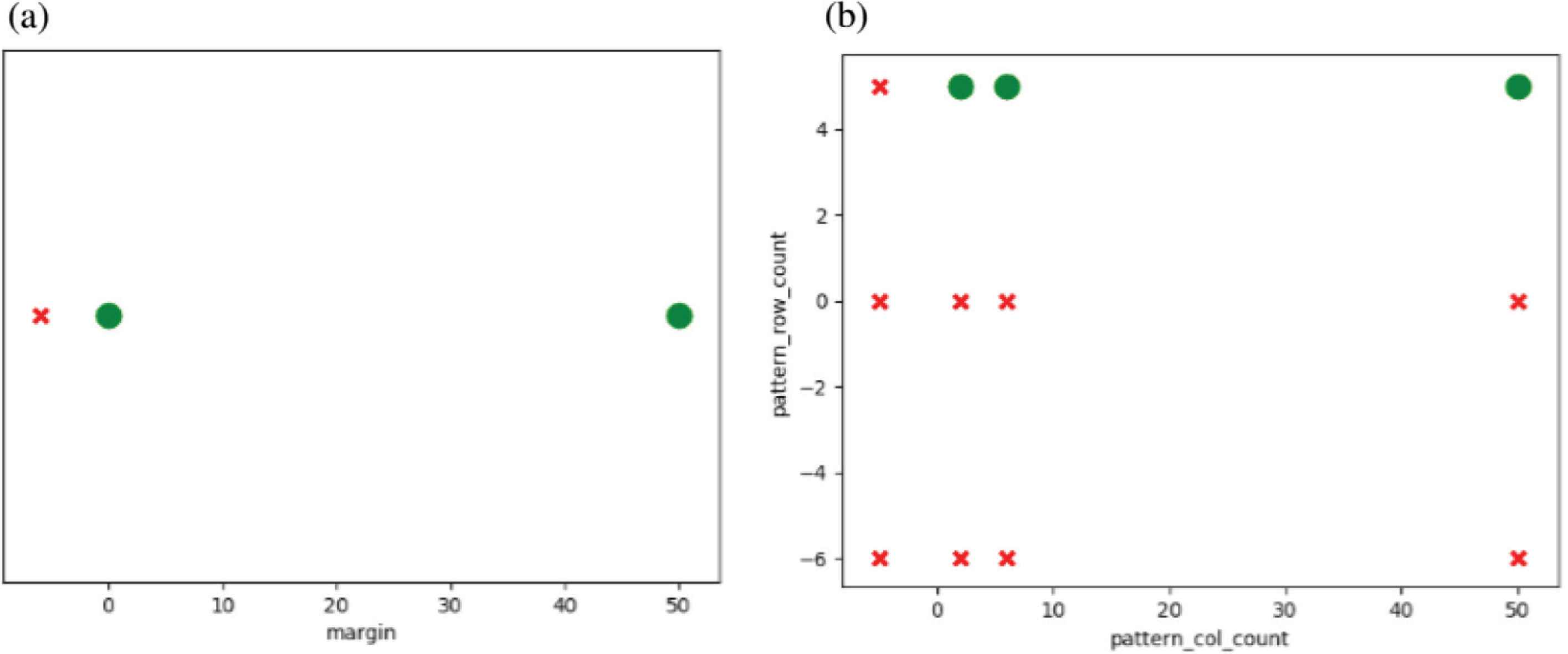
Parameters analysis.
These graphs represent the valid regions of each of the parameters provided or requested for analysis. They help discover passing or failing regions within the parameters that are not valid, as will be illustrated next, and validate that these parameters’ ranges follow the provided specifications. For the first graph, the margin parameter is analyzed, where the valid ranges were plotted as green circles, while invalid ranges were plotted as red crosses. It is clear that values beneath zero are invalid, while zero and above are acceptable. This was one of the mistakes captured by the MFSD, as the specifications provided for the tool stated that margin values should allow negative values. The second graph represents two parameters together (row and column counts), which shows that both of their ranges should be above zero to provide acceptable results.
5.2. xCalibrate™
xCalibrate™ is a software tool that allows the description of process technology information and generates a rule file containing Standard Verification Rule Format (SVRF) capacitance and resistance statements. The xCalibrate™ tool automatically creates the necessary capacitance and resistance rules for accurately extracting parasitic devices. The generated rule files can be included in a larger SVRF rule file for use by the Calibre® xACT, Calibre® xRC, and Calibre® xL tools during parasitic extraction [20]. This tool is different from the first tool because the input is not a set of parameters, but a file containing certain rules. However, MSFD allows template parsing of a template containing the keywords for the parameters to be replaced, along with their ranges. Random sampling of the parameters’ ranges is carried out, producing all the possible combinations of these templates to be fed into xCalibrate™. Seven parameters were sampled in xCalibrate™, producing 10,800 logs. Like the LSG, TF-IDF was applied on the output logs to produce numerical vectors, each containing 149 elements that were then fed into the neural network classifier model. In training the neural network, 2000 logs were used (1000 passing logs and 1000 failing logs). The training data was split between 80% training and 20% test data. Again, due to the discriminating features captured by the TF-IDF, the network reached an accuracy of 100% on the test data. After reapplying the TF-IDF to the failing logs, unsupervised mean-shift clustering was applied, producing numerical vectors each of length 94 elements. Eight failing regions were captured. Figure 9 shows the graph representing the logs for these regions after reducing the number of features from 94 to 2.
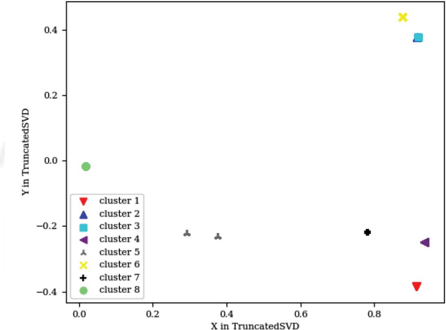
xCalibrate™ failing logs
xCalibrate™ was a different way to test MSFD because of the difference in input mentioned above, and because not all errors of the tool are clearly mentioned in the logs, as with the LSG. Although some of these errors were not captured by the logs, MSFD was able to cluster them successfully together, which proved the MSFD decision is not dependent upon the content of the log alone as much as the contents of all the logs together. When analyzing the failures in the eight clusters, one of the failing clusters contained three different failures because they were very close to each other, while all the other failing logs were totally different. That is, the failing logs of most of the clusters contained different formats from each other for displaying the errors. The close failures for the one cluster meant that its logs contained different error messages, but with a very similar display format. Such behavior was detected when the visualization of the graph provided in Figure 9 was zoomed in (the light green circular cluster, cluster 8), as shown in Figure 10.
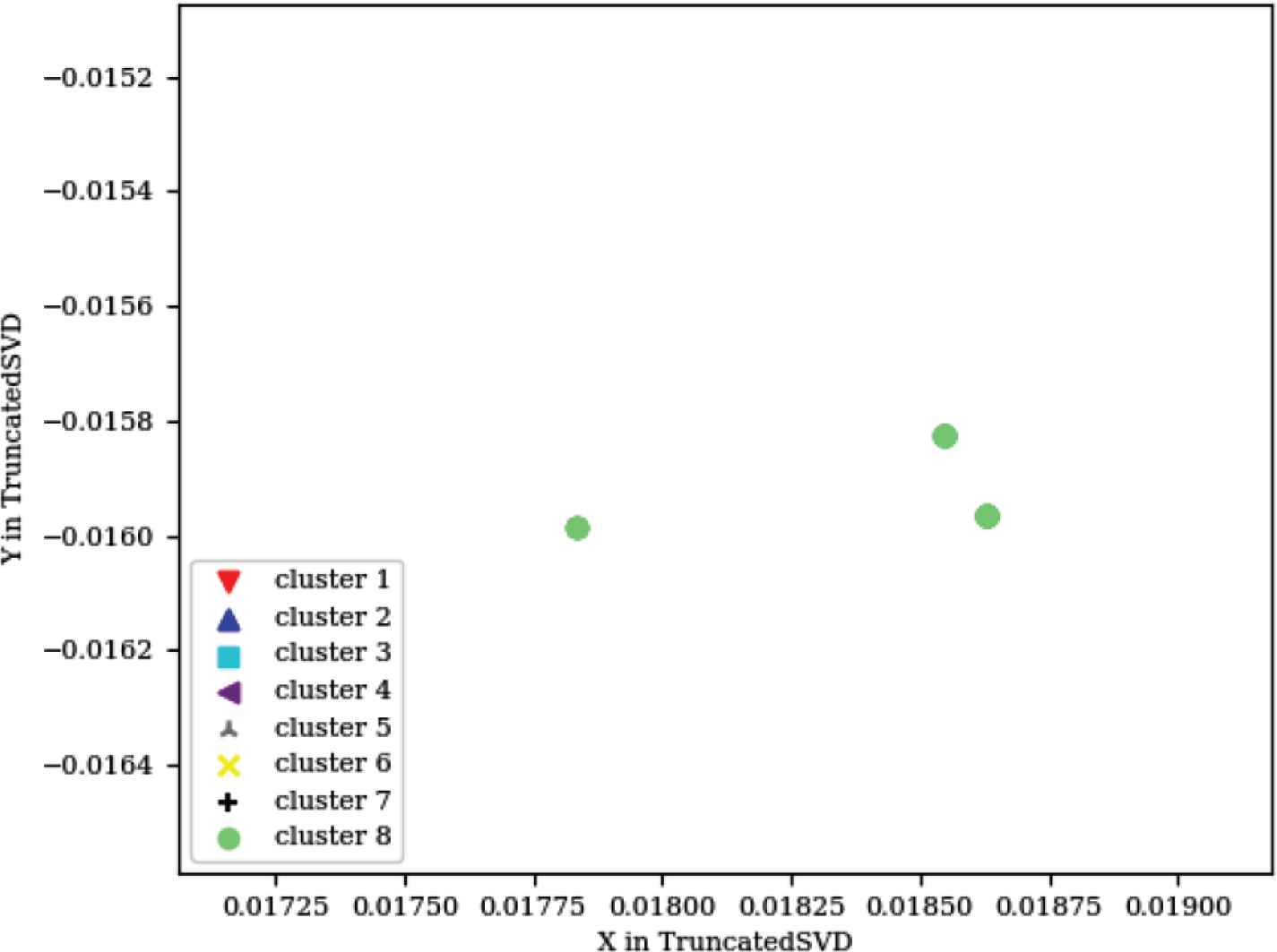
Zoomed in failing regions
However upon reapplying the mean-shift clustering on that cluster of logs alone, the three different clusters were separated successfully. Like the two final graphs for the LSG, Figure 11 represents the parameters that caused the failures in each of the clusters after being reduced to two dimensions from the seven dimensions provided (seven parameters were used), and Figure 12 shows a sample from the parameters being analyzed.
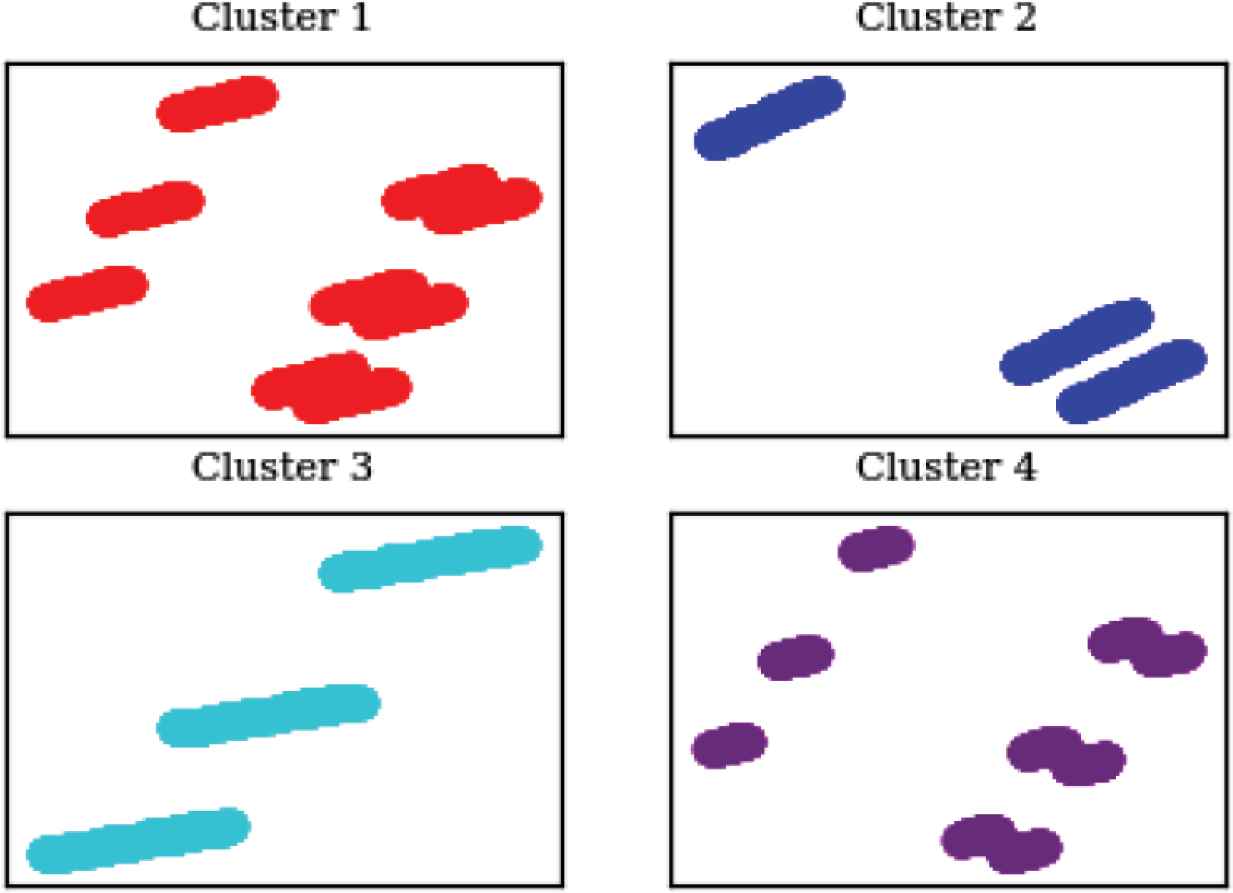
xCalibrate™ failing clusters parameters
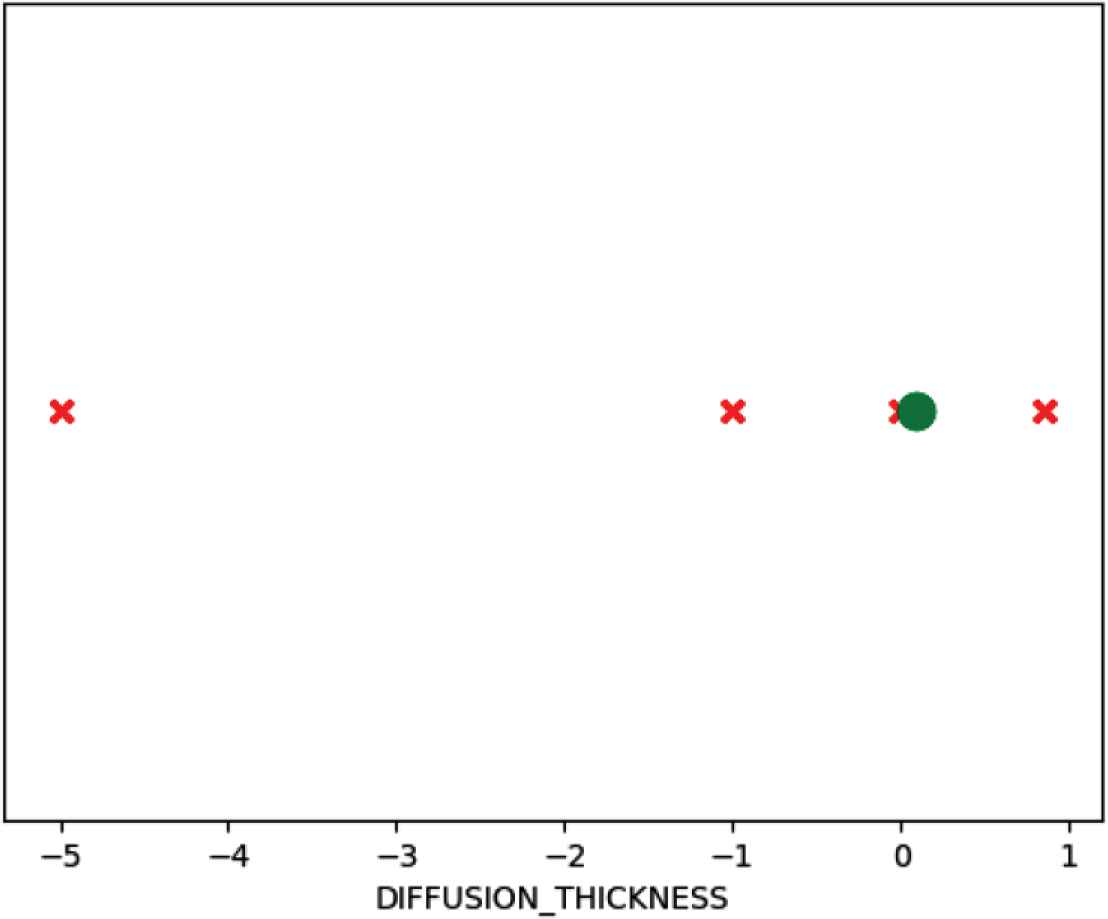
Diffusion thickness parameter
6. CONCLUSION
This paper proposed the MSFD tool for discovering the failing regions within a SUT, clustering similar failures together, visualizing the logs and the parameter values causing the failures, and plotting the acceptable ranges for each parameter or combination of two parameters. The input to MSFD was the list of ranges for the values of the parameters, passing through the parameters combination generation block, the feature extraction and machine learning block, and ending with the visualization. It was found that using TF-IDF in log analysis followed by a feed-forward ANN dramatically decreases both the depth of the ANN needed and the number of the training data, while providing accurate results. Using TF-IDF again on the failing logs allows the mean-shift clustering to perfectly cluster the logs. Our experiments with two different tools demonstrated the practicality of this approach for introducing automation into failure regions detection and parameters analysis.
CONFLICTS OF INTEREST
The authors declare they have no conflicts of interest.
REFERENCES
Cite this article
TY  - JOUR
AU  - Saeed Abdel Wahab
AU  - Reem El Adawi
AU  - Ahmed Khater
PY  - 2019
DA  - 2019/12/24
TI  - Machine Learning in Failure Regions Detection and Parameters Analysis
JO  - International Journal of Networked and Distributed Computing
SP  - 41
EP  - 48
VL  - 8
IS  - 1
SN  - 2211-7946
UR  - https://doi.org/10.2991/ijndc.k.191204.001
DO  - 10.2991/ijndc.k.191204.001
ID  - Wahab2019
ER  -