1. INTRODUCTION

Stabilities of feedback control systems are guaranteed under the assumption that the feedback loops are healthy. Obviously, if just one loop has a failed sensor, then the control system would lose its stability. Hence, detection for sensor failures plays an important role in maintaining the control system. In the previous works, several types of the Self-Repairing Control Systems (SRCS) have been developed against unknown sensor failures [1,2]. The SRCS can automatically detect failures, and replace failed sensors with healthy backups so as to maintain the system stability. Compared with existing active fault tolerant controls, the SRCS has the following advantages: (1) the detection filter has a simple structure that does not depend on the mathematical model of the plant, and (2) the maximum time for detection can be specified arbitrarily in advance, i.e., early fault detection can be attained. However, because unstable detection filters have been used [1], the conventional SRCS have been contrary to the concept of the strong stability, which claims that control systems should be constructed by stable elements [3].

In this paper, for the SRCS against sensor failures, a new design method for the detection filter is presented based on the simple spiking neuron model by Izhikevich [4], and also a concrete failure detection by counting the number of spikes in the filtered signal is shown. This method satisfies strong stability concept, because the filtered signal is always bounded. Furthermore, this paper shows the high-gain feedback controller stabilizing both the plant and the detection filter. It is shown that the overall control system has high robustness with respect to disturbances.

Throughout this paper, with x ∈ ℝ, we define the ‘sgn’ function by

Notice that this is slightly different from the ordinary one.

2. SPIKING NEURON MODEL

The spiking neuron model proposed by Izhikevich [4] is represented as [Equations (1) and (2)]:

where v ∈ ℝ is the membrane potential of the neuron, w ∈ ℝ is the recovery variable, I ∈ ℝ is the stimulus, and ε ∈ ℝ and γ ∈ ℝ are the parameters for the recovery dynamics. The auxiliary after-spike resetting is expressed by (2), where v_R ∈ ℝ and w_R ∈ ℝ are the reset values.

Figure 1 shows the well-known ‘bursting’ pattern with the parameters ε = 0.02, γ = 0.2, v_R = −50, w_R = 2, the initial values v(0) = −50, w(0) = 2 and the stimulus I = 10 [mV]. In both figures, ‘A’ indicates the first point where the auxiliary resetting (2) is performed.

Figure 1

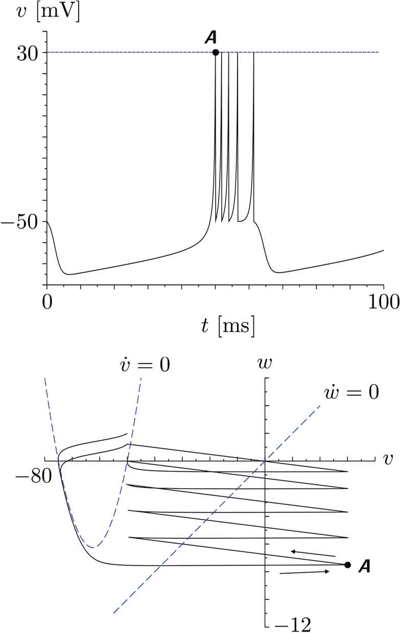
A ‘bursting’ pattern by Izhikevich spiking neuron model: the time history (top) and the trajectory (v, w) of the v – w plane (bottom).

Clearly, it is shown that each spike is shaped by the auxiliary resetting. This will be used for the fault detection of the proposed SRCS.

3. PROBLEM STATEMENT

Consider the following linear time invariant system with unknown disturbances.

where y ∈ ℝ is the actual output, u: ℝ⁺ → ℝ is the control input, and z ∈ ℝⁿ⁻¹ is the state. Also, d_y ∈ ℝ and d_z ∈ ℝⁿ⁻¹ are unknown but bounded disturbances. Here, it is assumed that the high frequency gain b ∈ ℝ is positive, and that F ∈ ℝ^{(n−1)×(n−1)} is the stable matrix (i.e., all eigenvalues lie in ℂ⁻).

For measurement of the output y, two sensors are prepared. One is the primary sensor #1, and the other is the backup #2 for occasion of failure. Then, the feedback signal y_s: ℝ⁺ → ℝ can be expressed as follows [Equation (4)].

where t_D ∈ ℝ⁺ is the detection time, whose details will be discussed later. Each y_i ∈ ℝ, i ∈ {1,2} is the output of the sensor #i. The healthy sensor output is y_i = y. Based on dynamic redundancy (4), we usually use the primary sensor #1, but switch to the backup #2 when the failure of the primary one is detected.

The failure scenario to be considered here, is expressed as follows [Equation (5)]:

where t_F ∈ ℝ⁺ is the unknown failure time, and φ ∈ ℝ is the unknown stuck value.

The aim of this paper is to design the SRCS, which can replace the failed sensor with the backup to maintain the control stability and guarantee the convergence property of y:

for arbitrarily given λ ∈ ℝ⁺.

4. CONTROL SYSTEM DESIGN

First of all, the detection filter is introduced based on the spiking neuron model expressed by (7) and (8).

where θ₀ ∈ ℝ, θ₁ ∈ ℝ, θ₂ ∈ ℝ, γ₀ ∈ ℝ, γ₁ ∈ ℝ, σ ∈ ℝ⁺ and η ∈ ℝ⁺ are design parameters. Also, v_T ∈ ℝ is the threshold for the auxiliary resetting. These parameters can be selected by scaling of the Izhikevich model parameters (see Section 6). For stability, the rule (8) of the resetting should be invalid before steady state, and then become valid after a sufficiently long control time.

Comparing the detection filter with the Izhikevich model, we can find that the part of the output feedback, ẏ_s + py_s in (7) corresponds to the stimulus I in (1). Furthermore, because y_s takes negative values, the sign function sgn[y_s] is introduced.

Next, the high-gain feedback controller is designed by

where p ∈ ℝ⁺ is the feedback gain to stabilize the plant and the detection filter. The nonlinear part, - yS3-v3 is introduced to handle the nonlinearities in the filter (7) .

The overall control system is illustrated in Figure 2.

Figure 2

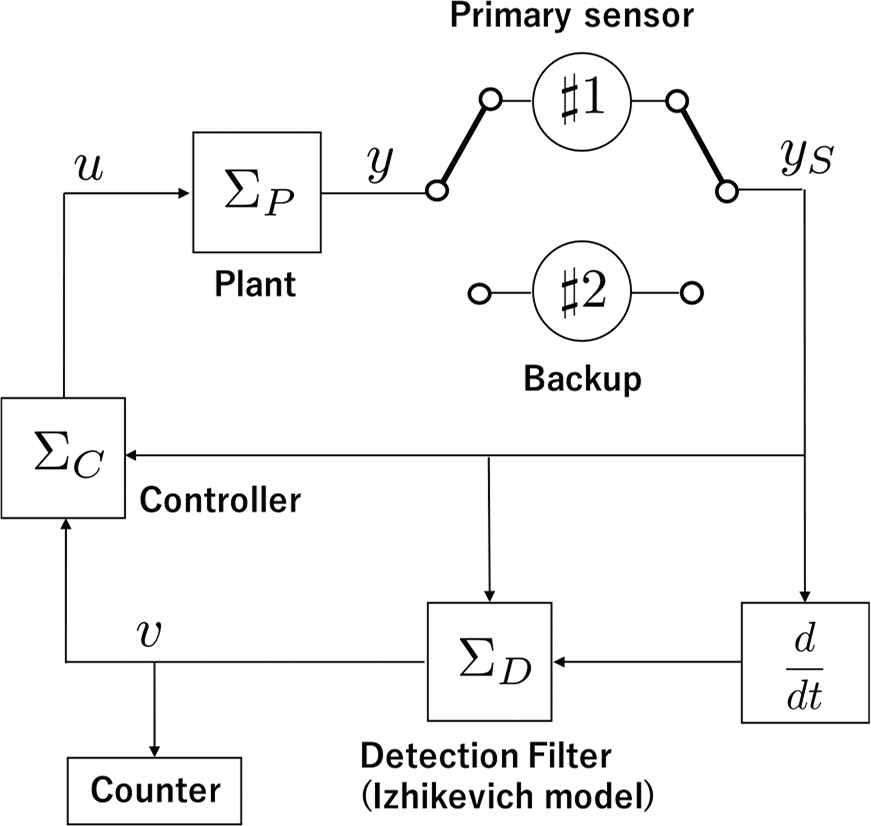
The block diagram of the proposed SRCS with the Izhikevich spiking neuron model.

Here, consider the case when the sensor is healthy, i.e., y_s = y. From (3), (7), and (9), the behavior of the overall control system without the auxiliary resetting (8) obeys

Define the positive definite function S: ℝ⁺ → ℝ⁺ as [Equation (11)] where P ∈ ℝ^{(n−1)×(n−1)} is the positive definite matrix which satisfies F^T P + P^T F = −2Q for any positive definite Q ∈ ℝ^{(n−1)×(n−1)}. Moreover, small constants δ > 0 and δ˜>0 are introduced only for analysis, i.e., these are not design parameters.

Taking the time derivative of S gives [Equation (12)]

where and d¯y≥|dy(t)|, d¯z≥ ∥dz(t)∥ . Choosing sufficiently large p, we have α_i > 0, i = 1, 2, 3. Hence, from (12) , it follows that where Solving the differential inequality (13), we have [Equation (15)] Therefore, we can conclude that all the signals in the control system are bounded in spite of existence of the disturbances. Moreover, if no sensor fails, that is, t_F = ∞, then we have [Equation (16)] For sufficiently small δ (sufficiently large p), we have 2δβ/α<λ . This means that the inequality (6) holds if no failure occurs.

With the same analysis, it can be verified that the filtered signal v also remains in a small region of radius λ, i.e., limt→∞sup|v|≤λ . Set the threshold as v_T > λ. Make the rule (8) of the resetting valid after a sufficiently long time. Then, spikes occur only during the failure, and no spike is induced whenever the sensor is healthy.

5. FAULT DETECTION

This section shows the concrete detection method using the detection filter given by (7) and (8).

Consider the case when the failure occurs. Then, the detection filter is represented as [Equation (17)]

This is similar to the Izhikevich model (1) . Refer to the ‘bursting’ as mentioned in Section 2. Roughly speaking, when the two nullclines in (1) are apart from each other (see the dashed blue lines, v.=0 and ẇ = 0 in Figure 1), the bursting pattern appears. Here, suppose that the parameters in (7) are chosen so that the following two nullclines are apart with a sufficient distance and never intersect. Then, from (8) and (17), it is shown that in the filtered signal v, the bursting pattern appears just like Figure 1. Hence, by monitoring the spikes in v, the failure can be detected. Thus, the detection time t_D is defined by where c_R ∈ ℕ is the number of the spikes in v, that is counted in real time, and n_R ∈ ℕ is the specified minimum number of spikes. Note that it is possible to count up the spikes from the number of times of the auxiliary resetting (8) in real time.

Because the occurrence time of the bursting can be arbitrarily shortened by selecting the parameters for the detection filter, the detection time can be hastened.

After replacing the failed sensor, the boundedness of all the signals in the control system are guaranteed again, and the convergence (6) can be obtained.

6. NUMERICAL EXAMPLES

To confirm the effectiveness of the proposed method, the numerical simulation is explored.

Consider the following plant with disturbances.

The initial values are y(0) = 1 and z(0) = −1.

In this example, the radius λ of the small region (6) to which the output y converges, is given by λ = 0.01.

The failure scenario (5) is supposed that

By the appropriate scaling of the bursting pattern shown in Figure 1, the parameters for the detection filter are selected as follows. These are chosen so that the bursting pattern of more than five spikes per second can be observed during sensor failure. Hence, by selecting n_R = 5, we can find the failure within almost 1 s. Thus, the detection time can be arbitrarily shortened.

To stabilize the plant and the detection filter mentioned above, by trial and error, the controller parameter is chosen as

Taking preliminary simulation results into account, the rule (8) of the auxiliary resetting is made valid from the beginning. Of course, no spike occurs whenever the sensor is healthy.

The simulation results are shown in Figure 3. In this figure, the measured output y_S, the actual output y (top) and the filtered signal v (bottom) are shown. From this result, it is clear that the control system can be well stabilized in spite of the existence of the disturbances, and the actual output y converges to a very small ball before and after the failure. The SRC can be accomplished, and the failed sensor is replaced at t_D ≅ 26 [s], i.e., early fault detection can be achieved by using the spiking neuron model.

Figure 3

Simulation results: the measured output and the actual output (top) and the filtered signal (bottom).

7. CONCLUSION

In this paper, the new SRCS has been developed that has the detection filter based on the spiking neuron model by Izhikevich. In this method, the sensor failure can be detected by counting the spikes in the filtered signal. The applications to nonlinear systems with noise, multiple-input and multiple output (MIMO) systems and so on are still left in the future works.

CONFLICTS OF INTEREST

The authors declare they have no conflicts of interest.

ACKNOWLEDGMENT

This work is supported by JSPS KAKENHI Grant Number JP16K06429.

Author Introduction

Dr. Masanori Takahashi

He received his B. Eng., M. Eng. and D. Eng. degrees from Kumamoto University, Japan in 1992, 1994 and 1998 respectively. He is currently a Professor with the Department of Electrical Engineering and Computer Science, Tokai University, Japan. His research interests are in the area of fault tolerant control, fault detection and adaptive control