
Evaluation of the Roller Arrangements for the Ball-Dribbling Mechanisms Adopted by RoboCup Teams
- DOI
- 10.2991/jrnal.k.191203.002How to use a DOI?
- Keywords
- The ball-dribbling mechanism; sphere slip velocity; sphere mobile speed efficiency
- Abstract
The middle-size league soccer competition is an important RoboCup event designed to promote advancements in Artificial Intelligence (AI) and robotics. In recent years, soccer robots using a dribbling mechanism, through which the ball is controlled using two driving rollers, have been adopted by teams worldwide. A survey conducted during the 2017 World Cup in Nagoya revealed that the teams determined their roller arrangements heuristically without the use of a formal mathematical process. In this study, we focus on sphere slip speed to develop a mathematical model for sphere rotational motion, allowing for slip. Using this framework, we derived the relationship between the sphere slip and mobile speeds and evaluated the roller arrangements used by the participating teams.
- Copyright
- © 2019 The Authors. Published by Atlantis Press SARL.
- Open Access
- This is an open access article distributed under the CC BY-NC 4.0 license (http://creativecommons.org/licenses/by-nc/4.0/).
1. INTRODUCTION
RoboCup is an international project that promotes innovation in Artificial Intelligence (AI), robotics, and related domains. It represents an attempt to develop AI and autonomous robotics research by providing a fundamental problem that can be solved by integrating a wide range of technologies. In particular, the middle-size league soccer competition is a RoboCup event providing a dynamical environment in which many robots cooperate with humans within the same space.
Various developments have been made in the RoboCup middle-size league soccer robot [1,2]. These robots generally have a mechanism similar to that of an omnidirectional movement mechanism using three-omni wheels [3] or that using four-omni wheels [4] and so on, and in recent years, this mechanism is involved in controlling the rotation of a ball. The ball holding mechanism is used.
In the past, several teams have equipped their robots such as arm type [5,6], bar type [7,8] and single-wheel type [9] with ball dribbling mechanisms for controlling the rotation of the ball. To be useful in soccer play, the dribbling performance of such mechanisms must be skillful. However, they cannot grasp a ball and control. Recently, dribbling devices use rollers to grasp the upper half of the ball to enable them to maintain a pull on it while driving in reverse. Friction is generated between the ball and rollers by a spring mounted on a supporting lever. To maintain dribbling, it is essential that the roller and ball rotate with approximately the same speed and that the ball moves in the same direction as the robot. Many robots, such as that deployed by the Turtles team [10], rely on ball handling force and use a roller arrangement in which there is slip between the roller and ball. To determine their roller arrangement, the Turtles rely on heuristic measures and experimental results. Although slip causes loss of speed in a moving sphere, the resulting friction can improve the ball holding power and rotational stability. Accordingly, slip is an important factor.
The authors conducted an investigation of the ball dribbling mechanisms employed by the teams at the 2017 middle-size league soccer competition in Nagoya, Japan. Table 1 lists our survey results, including team name and roller type, shape, and arrangement angle. The four shapes [◻⚪△◇] in the “Symbol” column indicate the roller angles used by the respective teams. Figure 1 shows the rotational axis, ball velocity, and roller velocity in reverse motion of a dual-roller arrangement. The RV-Infinity [11] roller arrangement in Table 1 involves no slip (see Figure 1a) because the roller velocity corresponds to the ball velocity; i.e., the rollers’ rotational axes are aligned on a plane that includes the origin of the ball’s sphere [12,13]. In another approach, CAMBADA [14] avoids slippage through the use of unconstrained rollers (omni-rollers).
| Team name | Symbol | Roller type | Angle |
|---|---|---|---|
| RV-infinity [11] | ◻ R | Constraint | 0° |
| The Turtles [10] | ⚪ T | Constraint | 10° |
| Falcons | ⚪ F | Constraint | 10° |
| Musashi150 [15] | △ H | Constraint | 20° |
| NuBot [16] | △ N | Constraint | 20° |
| Water | ◇ W | Constraint | 30° |
| CAMBADA | – | Unconstraint | 50° |
Survey result of roller type and angle in world teams
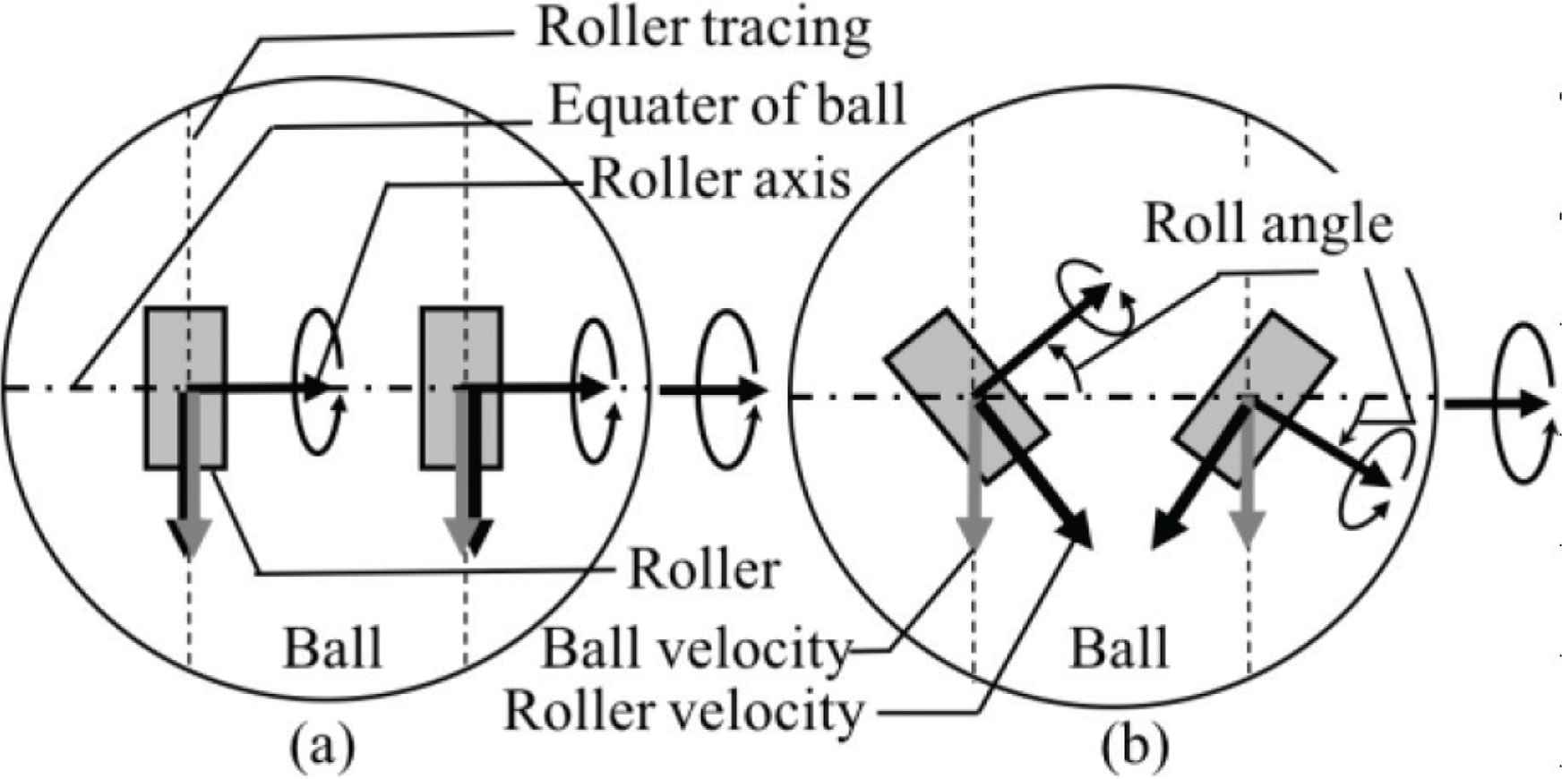
The ball reverse motion by two-rollers arrangement in the ball-dribbling mechanism. Case of (a) is zero-roller angle and case of (b) is non-zero-roller angle.
Other teams, namely the Turtles [10], Falcons, Musashi150 [15], NuBot [16], and Water, have adopted roller arrangements that allow for slip to occur (see Figure 1b) through a differential between roller and ball velocity. Based on analysis of sphere rotational motion in which slip is allowed, we developed a sphere kinematics model in which dual-constraint rollers allow for slipping [17].
In this study, we validated the model introduced in Kimura et al. [17] and evaluated the roller arrangements used by the competition teams from the standpoint of sphere speed, efficiency, and sphere slip speed (ball-holding power).
The remainder of this paper is organized as follows. In Section 2, we introduce a sphere kinematics model that allows for slipping. In Section 3, we validated the model introduced in Kimura et al. [17] and theoretical formula of sphere slip velocity vector. In Section 4, we considered the distribution of slip velocity vector and the roller arrangement of a ball dribbling mechanism based on the results of a robotic experiment. Finally, in Section 5, we present a summary and discuss future research.
2. THE SLIP VELOCITY VECTOR OF THE SPHERE
We quantify the slip between the sphere and roller.
As shown in Figure 2a, the center O of a sphere with radius r is fixed as the origin of the coordinate system ∑ − xyz. The i-th constraint roller is in point contact with the sphere at a position vector Pi and is arranged such that the center of mass of the roller PC, Pi and O are on the same line. ω denotes the angular velocity vector of the sphere. ηi denotes the unit vector along the rotational axis of constraint roller. νi the denotes peripheral speed of the constraint roller. αi (−90° ≤ αi ≤ 90°) denotes roller arrangement angle between ηi and span{P1, P2} which has unit normal vector e. The great circle CG passes thorough P1 and P2 are on the sphere. Normal orthogonal base {Xi, e} exist on the tangent plane span{Xi, e} at the Pi (see Figure 2b and 2c).
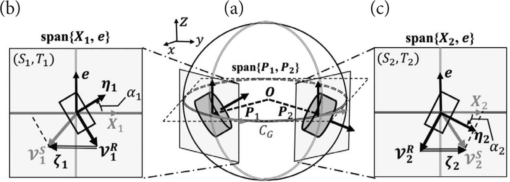
The existence of sphere slip velocity vector. (a) Isometric view. (b) Left side roller on span{X1, e}. (c) Right side roller on span{X2, e}.
3. VERIFICATION OF THEORETICAL FORMULA
In this chapter, we verified theoretical formulas including sphere kinematic (Section 3.1) and sphere slip velocity vector (Section 3.2) in reverse motion.
As shown in Figure 3, the conditions are given as follows: θ1,1 = 215°, θ1,2 = 325°, θ1,2, θ2,2 = 60°, r = 0.1 (m), α1 = α, α2 = −α (symmetry roller arrangement). Five experiments were conducted, each at the same four different degrees angles (α = 0°, 10°, 20°, 30°).

The location of contacted rollers on sphere for experiment. (a) Top view. (b) Back view.
3.1. Verification of Kinematics
As shown in Table 2, ||V||, φ and ρ are values calculated from v1, v2 = −0.91 (m/s) by Equations (11) and (14) refer to Kimura et al. [17].
| α | 0° | 10° | 20° | 30° |
| ||V|| (m/s) | 1 | 0.98 | 0.93 | 0.84 |
| φ (°) | −90 | −90 | −90 | −90 |
| ρ (°) | 0 | 0 | 0 | 0 |
Values calculated from v1, v2 = −0.91 (m/s)
3.1.1. Inverse kinematics
Figures 4–7 exhibit the theoretical data

Comparison theoretical value
Comparison theoretical value and experimental value in α = 10°.
Comparison theoretical value and experimental value in α = 20°.
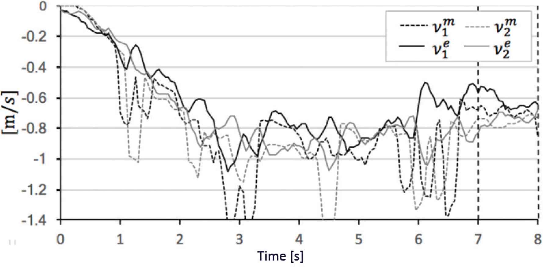
Comparison theoretical value and experimental value in α = 30°.
| 1 | 2 | 3 | 4 | 5 | |
|---|---|---|---|---|---|
| 0.03 | 0.04 | 0.10 | 0.10 | 0.03 | |
| 0.03 | 0.04 | 0.02 | 0.04 | 0.04 |
Absolute mean error [7–8 (s)] in α = 0°
| 1 | 2 | 3 | 4 | 5 | |
|---|---|---|---|---|---|
| 0.04 | 0.03 | 0.08 | 0.03 | 0.02 | |
| 0.03 | 0.04 | 0.01 | 0.04 | 0.04 |
Absolute mean error [7–8 (s)] case of α = 10°
| 1 | 2 | 3 | 4 | 5 | |
|---|---|---|---|---|---|
| 0.05 | 0.05 | 0.06 | 0.09 | 0.07 | |
| 0.03 | 0.03 | 0.05 | 0.06 | 0.05 |
Absolute mean error [7–8 (s)] case of α = 20°
| 1 | |
|---|---|
| 0.08 | |
| 0.05 |
Absolute mean error [7–8 (s)] case of α = 30°
In the evaluation case of α = 0°,
In the evaluation case of α = 10°,
In the evaluation case of α = 20°,
In the evaluation case of α = 30°, the limitations of the motor drivers and intense dynamical friction that caused heat between the roller surfaces and the sphere obliged us to cease the second and subsequent experiments. However, ||V||e, φe and ρe are partially close to ||V||m, φm and ρm, respectively (see Figure 7). And,
Thus, inverse kinematics is validated.
3.1.2. Forward kinematics
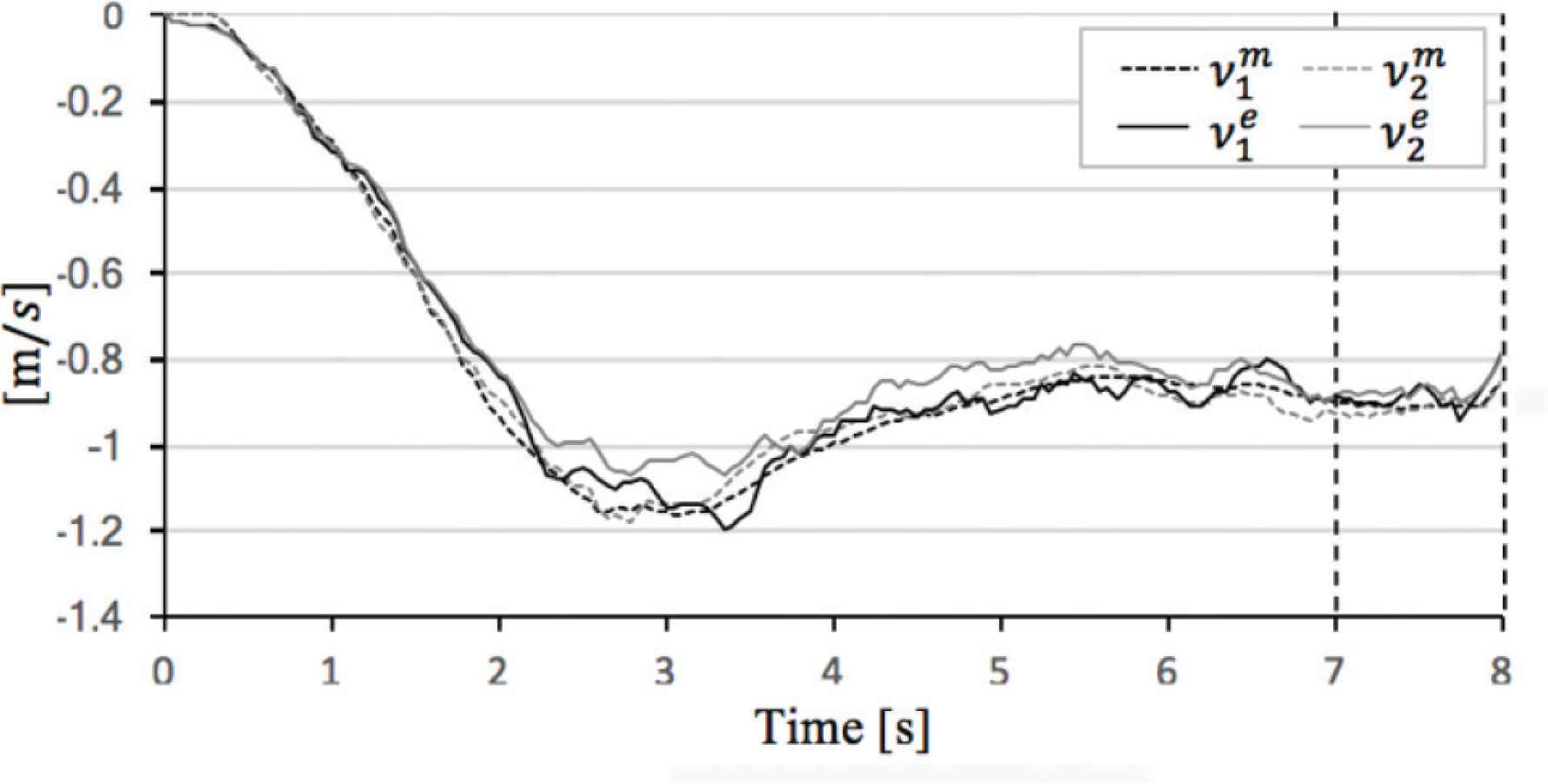
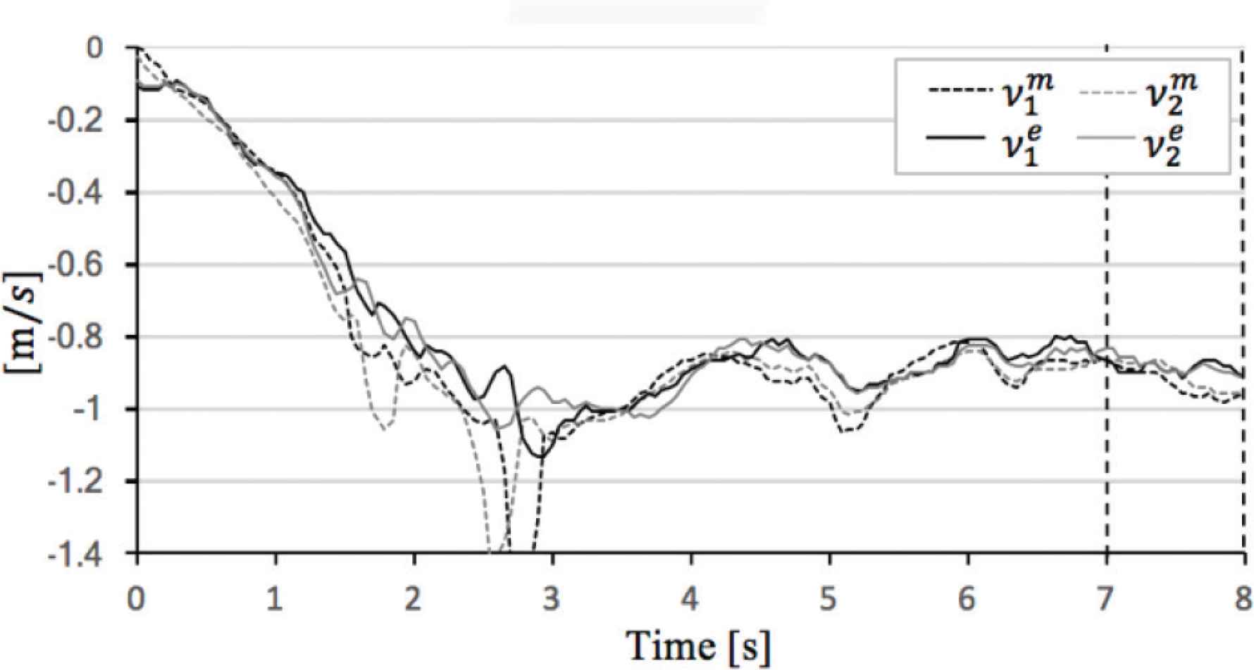
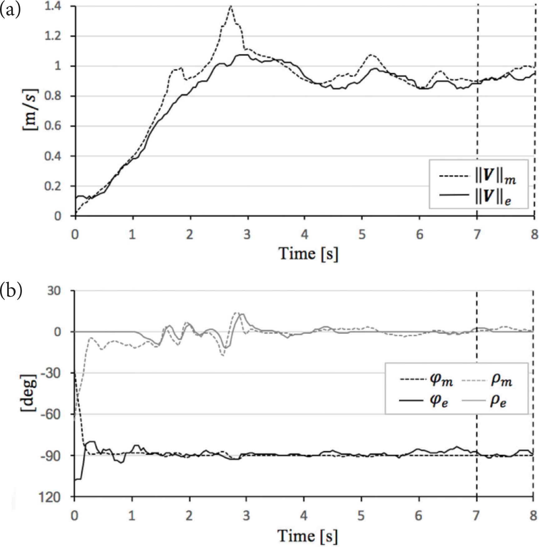
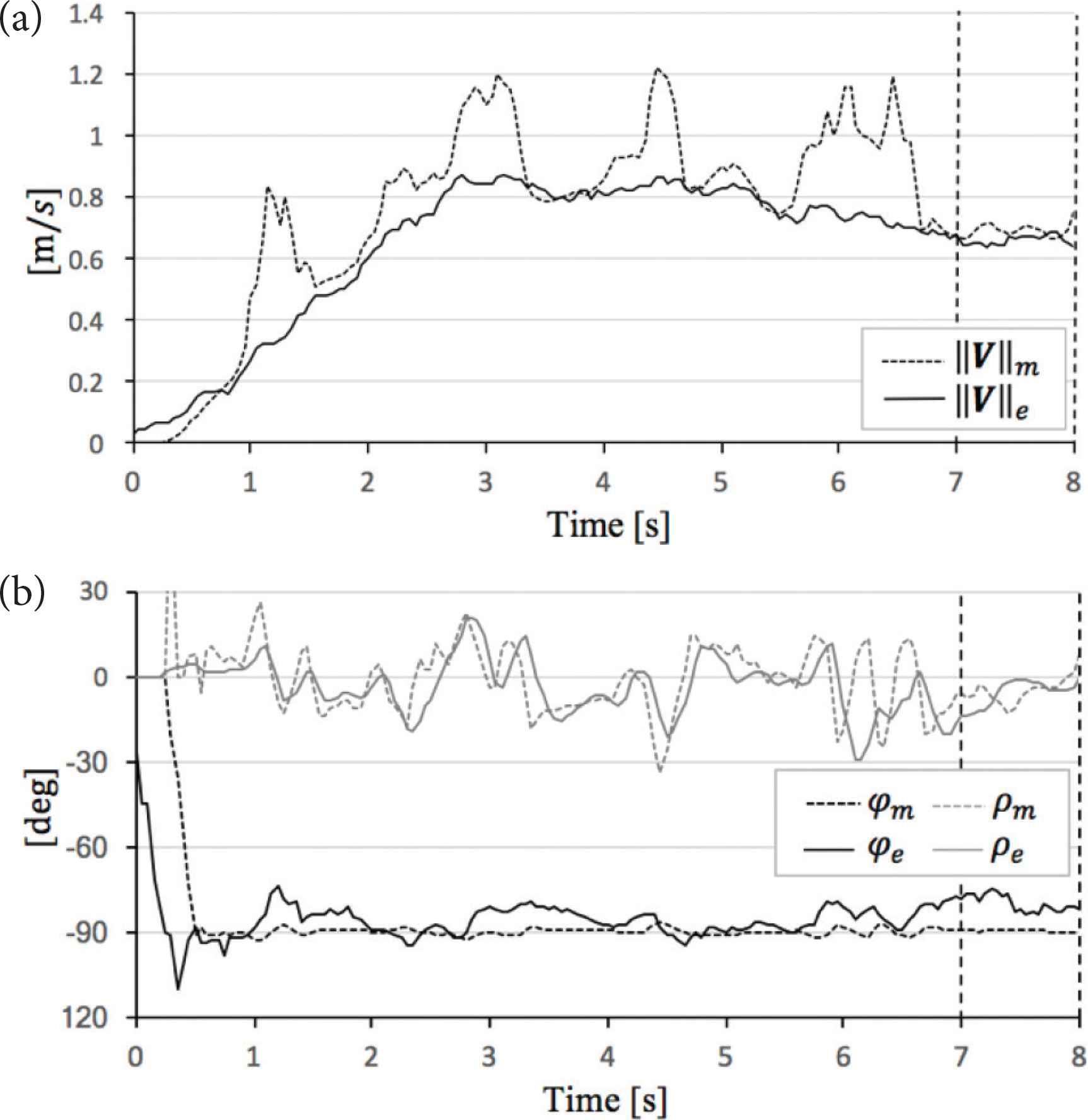
Figures 8–11 exhibit the theoretical data ||V||m, φm, ρm and experimental data ||V||e, φe, ρe. And, Tables 7–10 show the absolute mean error calculated in interval of 7–8 (s). We consider comparison between ||V||m, φm, ρm and ||V||e, φe, ρe, respectively in detail, see below.
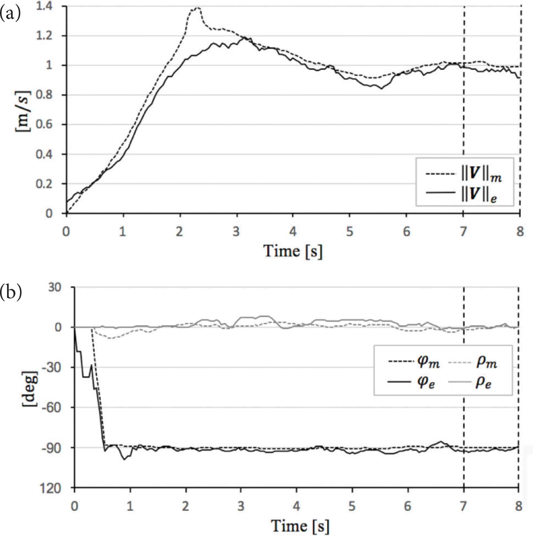
Comparison theoretical value and experimental value in α = 0°. (a) Sphere mobile speed. (b) Sphere direction and angle of sphere rotational axis.

Comparison theoretical value and experimental value in α = 10°. (a) Sphere mobile speed. (b) Sphere direction and angle of sphere rotational axis.
Comparison theoretical value and experimental value in α = 20°. (a) Sphere mobile speed. (b) Sphere direction and angle of sphere rotational axis.
Comparison theoretical value and experimental value in α = 30°. (a) Sphere mobile speed. (b) Sphere direction and angle of sphere rotational axis.
| 1 | 2 | 3 | 4 | 5 | |
|---|---|---|---|---|---|
| |||V||m − ||V||e| (m/s) | 0.03 | 0.04 | 0.05 | 0.06 | 0.04 |
| |φm − φe| (°) | 1.5 | 1.6 | 2.2 | 3.9 | 0.8 |
| |ρm − ρe| (°) | 0.7 | 0.9 | 6.3 | 5.3 | 0.9 |
Absolute mean error [7–8 (s)] in α = 0°
| 1 | 2 | 3 | 4 | 5 | |
|---|---|---|---|---|---|
| |||V||m − ||V||e| (m/s) | 0.03 | 0.04 | 0.04 | 0.03 | 0.03 |
| |φm − φe| (°) | 1.2 | 1.8 | 3.1 | 2.2 | 2.0 |
| |ρm − ρe| (°) | 2.1 | 1.0 | 3.9 | 1.2 | 1.2 |
Absolute mean error [7–8 (s)] in α = 10°
| 1 | 2 | 3 | 4 | 5 | |
|---|---|---|---|---|---|
| |||V||m − ||V||e| (m/s) | 0.03 | 0.03 | 0.06 | 0.07 | 0.05 |
| |φm − φe| (°) | 1.5 | 2.3 | 2.7 | 2.7 | 4.3 |
| |ρm − ρe| (°) | 1.9 | 1.4 | 2.1 | 2.1 | 2.1 |
Absolute mean error [7–8 (s)] in α = 20°
| 1 | |
|---|---|
| |||V||m − ||V||e| (m/s) | 0.04 |
| |φm − φe| (°) | 9.7 |
| |ρm − ρe| (°) | 5.1 |
Absolute mean error [7–8 (s)] in α = 30°
| α | 0° | 10° | 20° | 30° |
|---|---|---|---|---|
| S1 (m/s) | 0 | −0.16 | −0.31 | −0.45 |
| T1 (m/s) | 0 | 0 | 0 | 0 |
| S2(m/s) | 0 | 0.16 | 0.31 | 0.45 |
| T2 (m/s) | 0 | 0 | 0 | 0 |
Values calculated from v1, v2 = −0.91 (m/s)
In the evaluation case of α = 0°, ||V||e, φe and ρe are close to ||V||m, φm and ρm, respectively (see Figure 8). As shown in Table 7, |||V||m − ||V||e| is 0.06 (m/s), |φm − φe| is 3.9 (°), and |ρm − ρe| is 6.3 (°).
In the evaluation case of α = 10°, ||V||e, φe and ρe are close to ||V||m, φm and ρm (see Figure 9). As shown in Table 8, |||V||m − ||V||e| is 0.04 (m/s), |φm − φe| is 3.1 (°), and |ρm − ρe| is 3.9 (°).
In the evaluation case of α = 20°, ||V||e, φe and ρe are close to ||V||m, φm and ρm, respectively (see Figure 10). As shown in Table 9, |||V||m − ||V||e| is 0.07 (m/s), |φm − φe| is 4.3 (°), and |ρm − ρe| is 2.1 (°).
In the evaluation case of α = 30°, the data have intense behavior due to limitations of the motor drivers. However, ||V||e, φe and ρe are partially close to ||V||m, φm and ρm, respectively (see Figure 11). And, |||V||m − ||V||e| is 0.04 (m/s), |φm − φe| is 9.7 (°), and |ρm − ρe| is 5.1 (°) (see Table 10).
Thus, forward kinematics is validated.
3.2. Consideration of Slip Velocity Vector
As shown in Table 11, Si (i = 1, 2) are values calculated from v1, v2 = −0.91 (m/s) by Equation (1).
Using Equation (2) as
Figures 12–15 exhibit the theoretical data
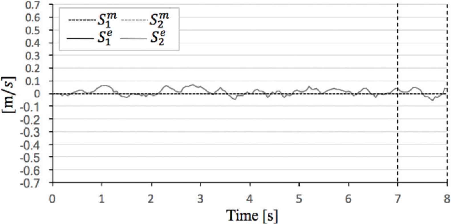
Comparison theoretical value and experimental value in α = 0°.
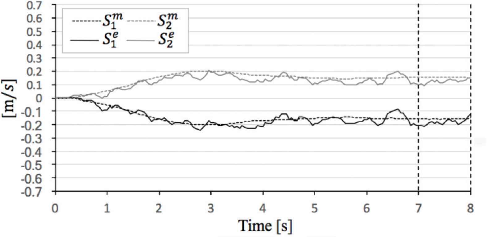
Comparison theoretical value and experimental value in α = 10°.
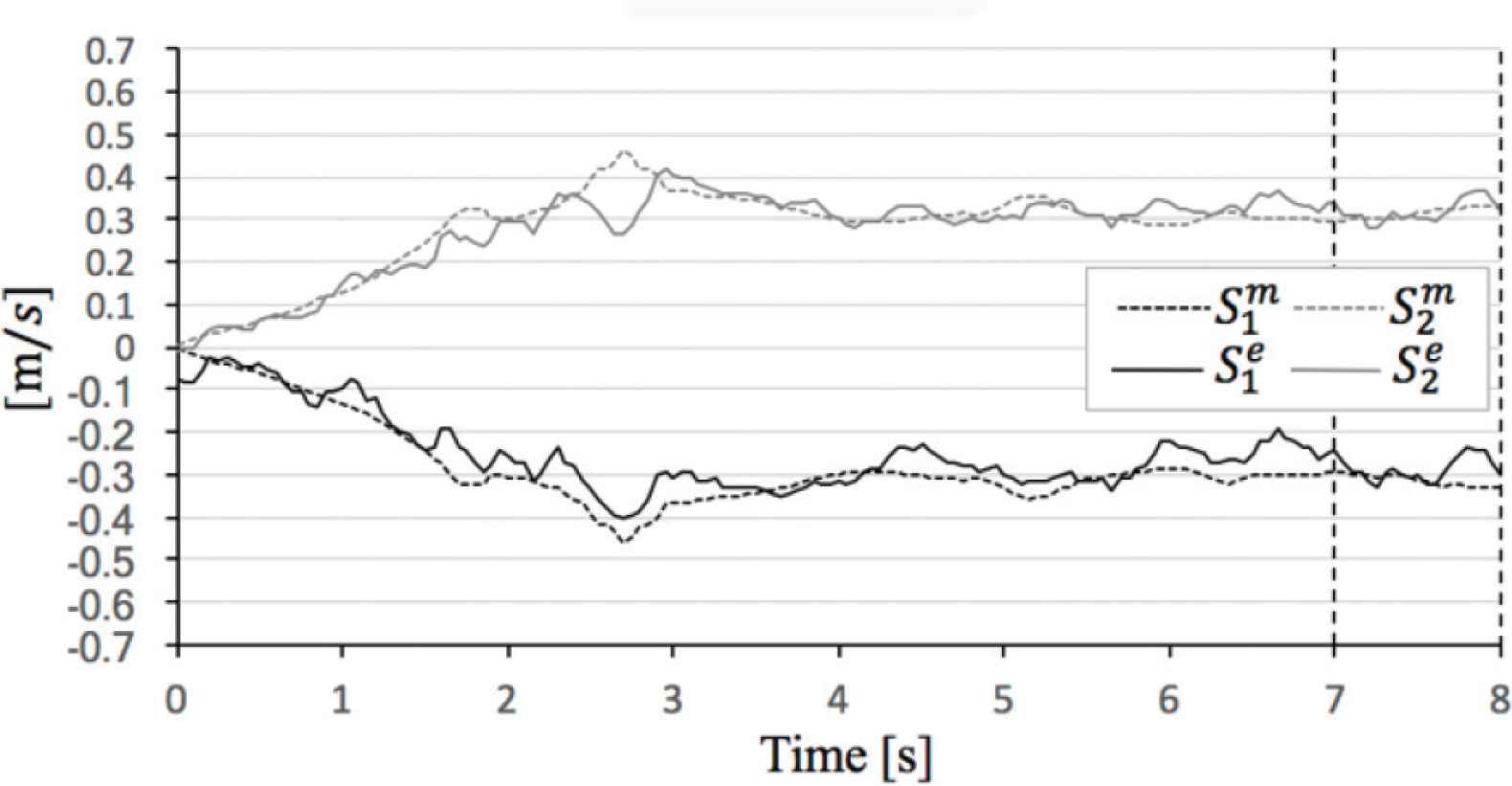
Comparison theoretical value and experimental value in α = 20°.
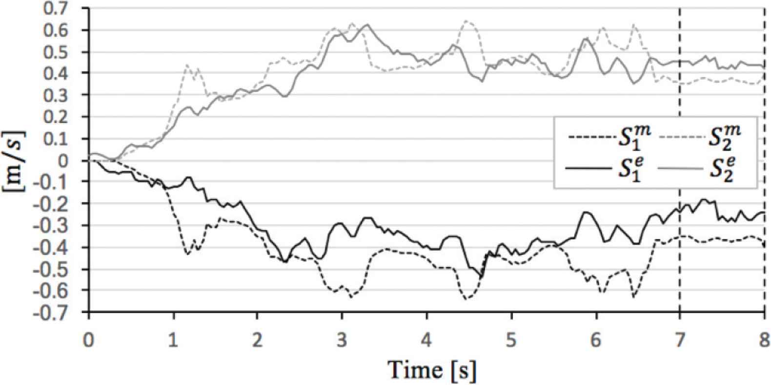
Comparison theoretical value and experimental value in α = 30°.
| 1 | 2 | 3 | 4 | 5 | |
|---|---|---|---|---|---|
| 0.02 | 0.03 | 0.02 | 0.04 | 0.01 | |
| 0.02 | 0.03 | 0.02 | 0.04 | 0.01 |
Absolute mean error [7–8 (s)] in α = 0°
| 1 | 2 | 3 | 4 | 5 | |
|---|---|---|---|---|---|
| 0.02 | 0.03 | 0.04 | 0.03 | 0.03 | |
| 0.02 | 0.03 | 0.03 | 0.04 | 0.03 |
Absolute mean error [7–8 (s)] in α = 10°
| 1 | 2 | 3 | 4 | 5 | |
|---|---|---|---|---|---|
| 0.03 | 0.04 | 0.06 | 0.05 | 0.09 | |
| 0.02 | 0.03 | 0.02 | 0.03 | 0.05 |
Absolute mean error [7–8 (s)] in α = 20°
| 1 | |
|---|---|
| 0.13 | |
| 0.08 |
Absolute mean error [7–8 (s)] in α = 30°
In the evaluation case of α = 0°,
In the evaluation case of α = 10°,
In the evaluation case of α = 20°,
In the evaluation case of α = 30°, the data have intense behavior due to limitations of the motor drivers. However,
Thus, Equations (1)–(3) is validated by experiment.
4. CONSIDERATION OF WORLD TEAMS’ ROLLERS ARRANGEMENT
Figure 16 shows the relationship between the sphere slip speed and sphere mobile speed. The horizontal and vertical axes show
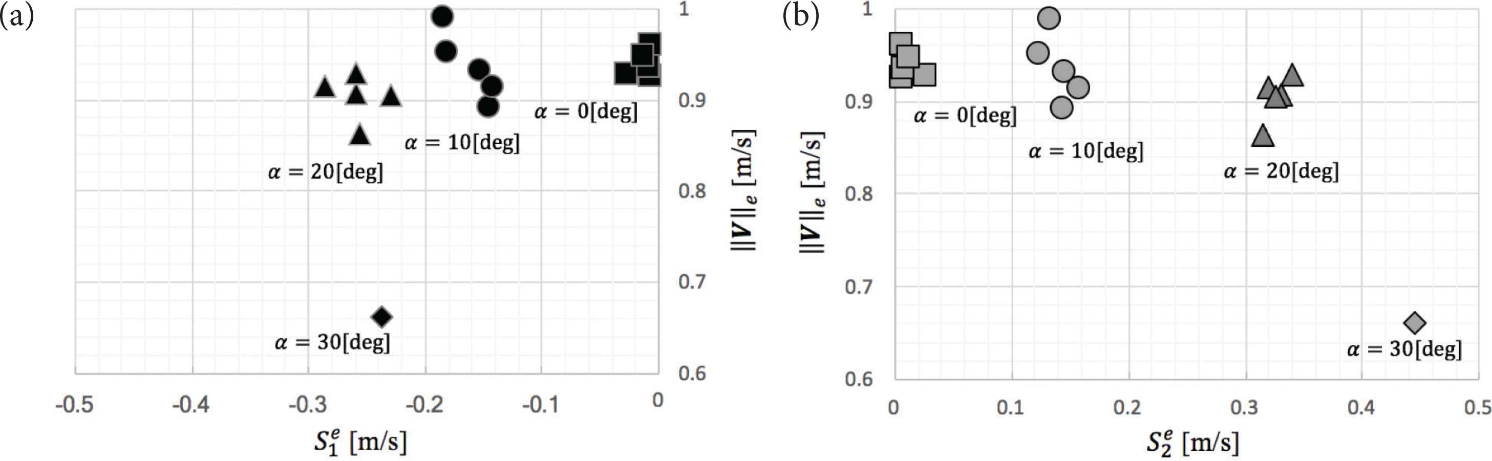
Relationship between sphere slip speed and sphere mobile speed. (a) Left-side roller. (b) Right-side roller.
The configurations  (left-side roller) and
  (right-side roller) indicate the coordinates
4.1. Vertical Coordinate (Mobile Speed)
For [ ] and [
 ], the sphere mobile speeds ||V||e are closely distributed within a range from 0.89 to 0.98 (m/s). The corresponding distributions of ||V||e for [
 ] are within the ranges from 0.86 to 0.92 (m/s) and [
 ] are 0.66 (m/s). Thus, [] and [] have the highest spherical speed efficiencies.
4.2. Horizontal Coordinate (Sphere Slip Speed)
For [], the values of ], [], and [] are mostly within the ranges from 0.13 to 0.18 (m/s), 0.23 to 0.34 (m/s), and 0.24 to 0.45 (m/s), respectively.
Under this kinematics model, it assumed that the roller and sphere contact at a single point. In reality, of course, they would contact along a surface, causing, ζi to generate a frictional force Fi in opposition to ζi. Referring to consideration, in which ζ1 and ζ2 are aligned back-to-back along a great circle, the frictional forces F1 and F2 generated by ζ1 and ζ2, respectively, would be in and are opposite directions and face-to-face (from Section 3 refer to Kimura et al. [17]).
For [] and [], there is an above-moderate frictional force. The [] and [] configurations adopted by RV-infinity, the Turtles, and the Falcons have the highest sphere speed efficiencies. However, [], the RV-infinity roller configuration, has nearly no friction [] adopted by the Turtles and Falcons has moderate friction [
Thus, by adopting [], the Turtles and Falcons have developed roller systems with the optimum arrangement at α = 10°.
5. CONCLUSION
In this study, we verified derive the sphere kinematics that allows for slipping and considered sphere slip velocity vector and evaluated the roller arrangement used by the world teams. As a result, Tech United Turtles and Falcons have adopted optimum roller arrangement in teams of mobile speed efficiency.
In future studies, by applying the ball-dribbling mechanism, this model should be verified experimentally.
CONFLICTS OF INTEREST
The authors declare they have no conflicts of interest.
Authors Introduction
Mr. Kenji Kimura
 He received the ME (mathematics) from Kyusyu University in 2002. Then he was a mathematical teacher and involved in career guidance in high school up to 2014. Currently, he is an educator of International Baccalaureate Diploma Program (Mathematics: applications and interpretation, analysis and approaches) in Fukuoka Daiichi High School, and student in the doctoral program of the Kyushu Institute of Technology. His current research interests are spherical mobile robot kinematics, control for object manipulation.
Dr. Shota Chikushi
 He received the M.S. and D.S. degrees from the Department of Life Science and Systems Engineering, Kyushu Institute of Technology, Fukuoka, Japan, in 2012 and 2018, respectively. He is an Assistant professor in the Department of Precision Engineering, Graduate School of Engineering, University of Tokyo. From 2015 to 2018, he was an Assistant professor of the Nippon Bunri University, Oita, Japan. His research interests are motion control of a roller-driven sphere, design for autonomous omnidirectional mobile robot and operation support of disaster response robot in unmanned construction.
Dr. Kazuo Ishii
 He is a Professor in the Kyushu Institute of Technology, where he has been since 1996. He received his PhD degree in Engineering from University of Tokyo, Tokyo, Japan, in 1996. His research interests span both Ship Marine Engineering and Intelligent Mechanics. He holds five patents derived from his research. His lab got “Robo Cup 2011 Middle Size League Technical Challenge 1st Place” in 2011. He is a member of the Institute of Electrical and Electronics Engineers, the Japan Society of Mechanical Engineers, Robotics Society of Japan, the Society of Instrument and Control Engineers and so on
REFERENCES
Cite this article
TY  - JOUR
AU  - Kenji Kimura
AU  - Shota Chikushi
AU  - Kazuo Ishii
PY  - 2019
DA  - 2019/12/24
TI  - Evaluation of the Roller Arrangements for the Ball-Dribbling Mechanisms Adopted by RoboCup Teams
JO  - Journal of Robotics, Networking and Artificial Life
SP  - 183
EP  - 190
VL  - 6
IS  - 3
SN  - 2352-6386
UR  - https://doi.org/10.2991/jrnal.k.191203.002
DO  - 10.2991/jrnal.k.191203.002
ID  - Kimura2019
ER  -