Correlated bivariate noncentral F distribution; factorial experiment; linear regression; pretest test; power and size of tests
Abstract
The data generated by many factorial experiments are analyzed by linear regression models. Often the higher order interaction terms of such models are negligible (e.g., R. Mead, The Design of Experiments, Cambridge University Press, Cambridge, 1988, p. 368) although there is uncertainty around it. This kind of nonsample prior information (NSPI) can be presented by null hypotheses (cf. T.A. Bancroft, Ann. Math. Stat. 15 (1944), 190–204), and its uncertainty removed through appropriate statistical test. Depending on the level of the NSPI the unrestricted, restricted, and pretest (PTT) tests are defined. The sampling distributions of test statistics and power functions of the three tests are derived. The graphical and analytical comparisons of powers reveal that the PTT dominates over the other tests.
In many real-life applications, the data of factorial experiments are analyzed using linear regression models. Unlike the classical and cell mean models, the regression model based method has the advantage of fitting the model in the presence of missing values or even with unbalanced data. The regression model for the response, Y of a 23 factorial experiment without any replication can be written as
where β’s are unknown regression parameters and x1, x2, and x3 represent the coded level of factors 1, 2, and 3, respectively, each assuming value −1 or 1 for the absence and presence of the factor. It is commonly assumed that the error term ϵ∼N0,σ2, where σ2>0 is a unknown spread parameter.
Mead [1] and Hinkelmann and Kempthorne [2] discussed how the higher order interactions of factorial experiments are believed to be negligible. Kabaila and Tesseri [3] reinforced that this kind of believe on the higher order interactions is the basis for fractional factorial experiments. To make valid inference on the remaining parameters, the uncertainty in the assumption of negligible interactions of any order can be represented by a hypothesis and conduct an appropriate test to remove the uncertainty (cf. Bancroft [4]). Any such assumptions can be considered as the nonsample prior information (NSPI) and used in the formal inferences on the remaining parameters of the model. Hodges and Lehmann [5] discussed the use of prior information from previous experience in reaching statistical decisions. Kabaila and Dharmarathne [6] compared Bayesian and frequentist interval estimators in regression utilizing uncertain prior information.
In the classical approach inferences about, unknown population parameters are drawn exclusively from the sample data. This is true for both estimation of parameters and hypothesis tests. Use of reliable NSPI from trusted sources (cf. Bancroft [4]), in addition to the sample data, is likely to improved the quality of estimation and test. The use of NSPI has also been demonstrated by Kempthorne [7,8], Bickel [9], Khan [10–12], Khan and Saleh [13–15], Khan et al. [38] and Saleh [16].
Such NSPI is usually available from previous studies or experts in the field or practical experience of the researchers, and is independent of the sample data under study. The main purpose of inclusion of NSPI is to improve the quality of statistical inference. In reality, NSPI on the value of any parameter may or may not be close to the unknown true value of the parameter, and hence there is always an element of uncertainty. But the uncertain NSPI can be expressed by a null hypothesis and an appropriate statistical test can be used to remove the uncertainty. The purpose of the preliminary test (pretest) on the uncertain NSPI in the hypothesis testing or estimation is to improve the quality of the inference (cf. Khan [17]; Saleh [16]; Yunus [18]). Kabaila and Dharmarathne [6] and Kabaila and Tissera [3] used NSPI to construct confidence intervals for regression parameters. In this paper, we express the data from a factorial experiment as a linear model (see (1)) in order to test the coefficients of the main effects (and lower order interactions) when there is uncertain NSPI on the coefficients of higher level interactions.
The uncertain NSPI can be any of the following types: (i) unknown (unspecified)—NSPI is not available, (ii) known (certain or specified)—exact value is the same as the parameter, and (iii) uncertain—suspected value is unsure. In the estimation regime, to cater for the three different scenarios, the following three different estimators are appropriate: (i) unrestricted estimator (UE), (ii) restricted estimator (RE), and (iii) preliminary test estimator (PTE) (see eg Judge and Bock [19]; Saleh [16]).
Almost all of the works in this area are on the estimation of parameter(s). These include Bancroft [4,20], Han and Bancroft [21], and Judge and Bock [19] introduced the preliminary test estimation method to estimate the parameters of a model with uncertain NSPI. Later Khan [10–12], Khan and Saleh [14], and Khan and Hoque [22] covered various work in the area of improved estimation.
The testing of parameters in the presence of uncertain NSPI is relatively new. The earlier works include Tamura [23] and Saleh and Sen [24,25] in the nonparametric setup. Later Yunus and Khan [26–28] used the NSPI for testing hypothesis using nonparametric methods. The problem is yet to be explored in the parametric context. In this paper testing of hypotheses is considered on the coefficients of the main effects in the model in (1) when uncertain nonsample information on the coefficients of the higher order interactions is available.
To set up the hypotheses for the tests, let’s assume that the interaction terms (e.g., last four β′s) of model (1) are suspected to be zero, but not sure. Then under the three different scenarios define three different tests: (i) unrestricted test (UT), (ii) restricted test (RT), and (iii) pretest test (PTT) to test on the remaining regression parameters (first four β′s) of the model. The UT uses the sample data alone but the RT and PTT use both the NSPI and the sample data. The PTT is a choice between the UT and the RT.
The regression model and hypotheses are provided in Section 2. Some useful results are discussed in Section 3. The proposed test statistics and their sampling distributions are provided in Sections 4 and 5, respectively. Section 6 derives the power function and size of the tests. An example with real data is included in Section 7. The power of the tests are compared in Section 8. Some concluding remarks are provided in Section 9.
2. THE REGRESSION MODEL AND HYPOTHESES
The regression model for the data from a 23 factorial experiment, as stated in (1), can be viewed as special case of the multiple regression model where each of the main effect and interaction terms are represented as the explanatory variables. For an n set of observations on the response Y and k explanatory/independent variables X1,⋯,Xk, that is, Xij,Yi, for i=1,2,⋯,n and j=1,2,⋯,k, the linear model is given by
Yi=β0+β1Xi1+⋯+βkXik+ei,
where β′s are the regression parameters and ei’s are the error terms. The model in equation (2) can be here expressed following convenient form
Y=Xβ+e,
where β=β0,β1,⋯,βr−1,βr,⋯,βk′ is a column vector of order k+1=p, Y=y1,⋯,yn′ is vector of response variables of dimension n×1, X is an n×p matrix of full rank of the independent variables, and e is a vector of errors. It is assumed components e are identically and independently distributed as normal variable with mean 0 and variance σ2, so that e∼Nn0,σ2In, where In is an identity matrix of order n.
To formulate the testing problem, let δ1=β0,⋯,βr−1 be a subset of r regression parameters and δ2=βr,⋯,βk be another subset of p−r=s regression parameters, so that r+s=p. The regression vector β is then partitioned as β′=δ′1,δ′2, where δ′1 is a r dimensional sub-vector, and δ′2 is a subvector of dimension s=p−r. In a similar way, matrix X is partitioned as X1,X2 with X1=1,x1,⋯,xr−1, an n×r matrix, and X2=xr,⋯,xk, an n×s matrix. Then the multiple regression model in (3) can be written as
Y=X1δ1+X2δ2+e.
We wish to perform test on the subvector δ1 (or β1) when NSPI on the subvector δ2 (or β2) is available.
Depending on the nature of the NSPI on the subvector, δ2, to be (i) unspecified, (ii) specified (fixed), or (iii) suspected to be a specific value but not sure, we define three different tests for testing the other subvector, δ1. Let A1 be a q1×r matrix of constants and A2 be another q2×s matrix of constants, where q=q1+q2 so that
A=A1OOA2,
that is, A is a q×p matrix and O is a matrix of zeros. The NSPI on the value of δ2 is expressed in the form of a null hypothesis, H0*:A2δ2=h2. Then to test the null hypothesis H0:A1δ1=h1 against Ha:A1δ1≠h1.
The hypothesis defined here, H0:Aβ=h, that is,
H0:Aβ=A1OOA2δ1δ2=h1h2
is a generalization of the test of equality of components of the regression vector and the subhypothesis
H0:β1β2=δ1δ2=δ10
(cf. Saleh [16], pp. 340). Note that h2 is only used for the pretest on β2 (i.e., PT), as such its value remains the same when testing β1.
3. SOME PRELIMINARIES
To formally define the tests let us consider the following expressions, partitions and results. For the full rank design matrix X we write
X′X=X′1X1X′1X2X′2X1X′2X2,X′X−1=A11A12A21A22,
where
A11−1=X′1X1−X′1X2X′2X2−1X′2X1 and A22−1=X′2X2−X′2X1X′1X1−1X′1X2.
Then the unrestricted least squares estimator of the regression parameters is given by
β~=X′X−1X′Y=δ~1δ~2,
so that the UE of the two subvectors are
δ~1=A11X′1Y+A12X′2Y and δ~2=A22X′2Y+A21X′1Y.
Then the sum of square errors for the full regression model with k regressors is given by
SSEF=Y−Xβ~′Y−Xβ~,
so an unbiased estimator of σ2 is MSEF=SSEF/n−p.
Let δ2 be specified to be δ20, so the RE of β becomes,
β^=β^1β^2=δ^1δ^2=β~−C−1A′AC−1A′−1Aβ~−h,
where C=X′X. Since β~∼Npβ,σ2C−1, we get
δ~1∼Nrδ1,σ2A11−1δ~2∼Nsδ2,σ2A22−1.
Similarly, as β^∼Npβ,σ2D−1, where D=C−1−C−1A′AC−1A′−1AC−1−1, we get
δ^1∼Nrδ1,σ2D11−1δ^2∼Nsδ2,σ2D22−1,
in which
D=D11D12D21D22.
Since Aβ~ is linear combination of normal variables Aβ~∼NqAβ,σ2AC−1A′−1 and Aβ^∼NqAβ,σ2AD−1A′−1.
Furthermore, the test statistic for testing H0:A1δ1=h1 is given by
F*=1qse2A1δ~1−h1′A1X′1X1−1A′1−1A1δ~1−h1,
where se2=1n−pY−Xβ~′Y−Xβ~ is an unrestricted unbiased estimator of σ2.
It is clear that 1σ2A1δ~1−h1′A1C1−1A′1−1A1δ~1−h1, where C1=X′1X1, follows a noncentral chi-squared distribution with q1 degrees of freedom (df) and noncentrality parameter Δ12/2, where
Δ12=A1δ1−h1′A1C1−1A′1−1A1δ1−h1σ2.
Under Ha, the F* statistic follows a noncentral F distribution with q1,n−p df and noncentrality parameter Δ12/2, and under H0, F* follows a central F distribution with q1,n−p df. Ohtani and Toyoda [29] and Gurland and McCullough [30] also used the above F test for testing linear hypotheses.
4. THE THREE TESTS
For testing δ1 when NSPI is available on δ2, define the tests as
For the UT, let ϕUT be the test function and TUT be the test statistic for testing H0:A1δ1=h1, a vector of order q1, against Ha:A1δ1≠h1 when δ2 is unspecified,
For the RT, let ϕRT be the test function and TRT be the test statistic for testing H0:A1δ1=h1 against Ha:A1δ1≠h1 when δ2=δ02 (specified) and
For the PTT, let ϕPTT be the test function and TPTT be the test statistic for testing H0:A1δ1=h1 against Ha:A1δ1≠h1 when δ2 is suspected to be δ02 following a pretest (PT) on δ2. For the PT, let ϕPT be the test function for testing H0*:A2δ2=h2 (a suspected vector of order q2) against Ha*:A2δ2≠h2. If H0* is rejected in the PT, then the UT is used to test on δ1, otherwise the RT is used to test H0.
Then the proposed three test statistics are defined as follows:
The UT for testing H0:A1β1=h1 is given by
LUT=A1β1~−h1′A1X′1X1−1A′1−1A1β1~−h1qse2,
where se2 is the unbiased estimator of σ2. Under H0, LUT follows an F distribution with q1 and n−p df whereas under Ha the LUT follows a noncentral F distribution with q1,n−p df and noncentrality parameter Δ12/2.
The RT is given by
LRT=A1δ^1−h1′A1D11−1A′1−1A1δ^1−h1q1se2.
Under Ha, LRT follows a noncentral F distribution with q1,n−p df and noncentrality parameter Δ22/2, where
Δ22=A1δ1−h1′A1D11−1A′1−1A1δ1−h1σ2.
For the preliminary test on δ2, we test H0*:A2δ2=h2 against Ha*:A2δ2≠h2 using the statistic
LPT=A2δ2~−h2′A2A22−1A′2−1A2δ2~−h2q1se2,
where se2 is an unbiased estimator of σ2. Under Ha, LPT follows a noncentral F distribution with q2,n−p df and noncentrality parameter Δ32/2, where
Δ32=A2δ2−h2′A2D22−1A′2−1A2δ2−h2σ2.
Let αj0<αj<1, for j=1,2,3 be a positive number. Then set Fν1,ν2,αj, in which ν1 and ν2 are the numerator and denominator d.f., respectively, such that
PLUT>Fq1,n−p,α1|A1δ1=h1=α1,
PLRT>Fq1,n−p,α2|A1δ1=h1=α2,
PLPT>Fq2,n−p,α3|A2δ2=h2=α3.
To test H0:A1β1=h1 against Ha:A1β1≠h1, after pretesting on δ2, the test function is
Φ=1,ifLPT≤Fc,LRT>Fb or LPT>Fc,LUT>Fa;0,otherwise,
where Fa=Fα1,q1,n−p, Fb=Fα2,q1,n−p and Fc=Fα3,q2,n−p.
5. SAMPLING DISTRIBUTION OF TEST STATISTICS
The sampling distribution of the test statistics are discussed in this section. For the power function of the PTT the joint distribution of LUT,LPT and LRT,LPT are essential. Following Khan and Pratikno [31], let Mn be a sequence of alternative hypotheses defined as
Mn:A1β1−h1,A2β2−h2=λ1n,λ2n=λ,
where λq×2 is a vector of fixed real numbers. Under Mn both A1β1−h1 and A2β2−h2 are nonsingular matrices and under H0 they are singular matrices.
From Yunus and Khan [28] and (13), define the test statistic of the UT when δ2 is unspecified, under Mn, as
L1UT=LUT−nσq1se2A1β~1−h1′A1X′1X1−1A′1−1A1β~1−h1.
The statistic L1UT follows a noncentral F distribution with q1,n−p df and a noncentrality parameter which is a function of A1β1−h1.
From (14), under Mn, A1β1−h1 the test statistic of the RT becomes
L2RT=LRT−nσq1se2A1δ^1−h1′A1D11−1A′1−1A1δ^1−h1.
The statistic L2RT also follows a noncentral F distribution with q1,n−p df and a noncentrality parameter which is a function of A1β1−h1 under Mn. From (16) the test statistic of the PT is given by
L3PT=LPT−nσq2se2A2δ~2−h2′A2A22−1A′2−1A2δ~2−h2.
Under Ha, the L3PT follows a noncentral F distribution with q2,n−s df and a noncentrality parameter which is a function of A2β2−h2.
From (13), (14), and (16) we observe that the LUT and LPT are correlated, and that LRT and LPT are uncorrelated. The joint distribution of the LUT and LPT is a correlated bivariate F distribution with q1,n−p and q2,n−p df. The details on the bivariate central F distribution is found in Krishnaiah [32], Amos and Bulgren [33], and El-Bassiouny and Jones [34]. Khan et al. [35] provided the probability density function and some properties of correlated noncentral bivariate F distribution. The covariance and correlation of the correlated bivariate F distribution for the LUT∼F1q1,n−p and LPT∼F2q2,n−p are then given, respectively, as
where a=Fα3,q1,n−p−σqse2λ2′γpt−1λ2=Fα3,q2,n−p−kptζ2, and d1ra,b is bivariate F probability integral. The value of ζ1 and ζ2 depend on λ1 and λ2, respectively, and
with b=Fα1,q1,n−p−Ωut. The integral ∫0b∫0afFPT,FUTdFPTdFUT is the cdf of the correlated bivariate noncentral F (BNCF) distribution of the UT and PT. Following Yunus and Khan [36], we define the pdf and cdf of the BNCF distribution as
fy1,y2=mnm1−ρ2m+n2Γn/2∑j=0∞∑r1=0∞∑r2=0∞ρ2jmn2jΓm/2+j×e−θ1/2θ1/2r1r1!mnr1Γm/2+j+r1y1m/2+j+r1−1×e−θ2/2θ2/2r2r2!mnr2Γm/2+j+r2y2m/2+j+r2−1×Γqrj1−ρ2+mny1+mny2−qrj, and
FY1,Y2a,b=PY1<a,Y2<b=∫0a∫0bfy1,y2dy1dy2.
By setting a=b=d, Schuurmann et al. [37] presented the critical values of d for the probability table of multivariate F distribution.
From (30), it is clear that the cdf of the BNCF distribution involved in the expression of the power function of the PTT.
6.2. The Size of the Tests
The size of a test is the value of its power under the null hypothesis, H0. The size of the UT, RT, and PTT are given by
where h=Fα1,q1,n−p, d=Fα2,q1,n−p, and under H0 the value of a is Fα1,q1,n−p.
7. ILLUSTRATIVE EXAMPLE
To compare the tests, the properties of the three tests are studied using simulated data. The R statistical package was used to generate data on Y and X. Using k=3, three covariates xj,j=1,2,3 were generated from the U0,1 distribution. The error vector e was generated from the Nμ=0,Σ=σ2I3 distribution. For n=100 random variates the dependent variable y was determined by yi=β0+β1xi1+β2xi2+β3xi3+ei for i=1,2,⋯,n.
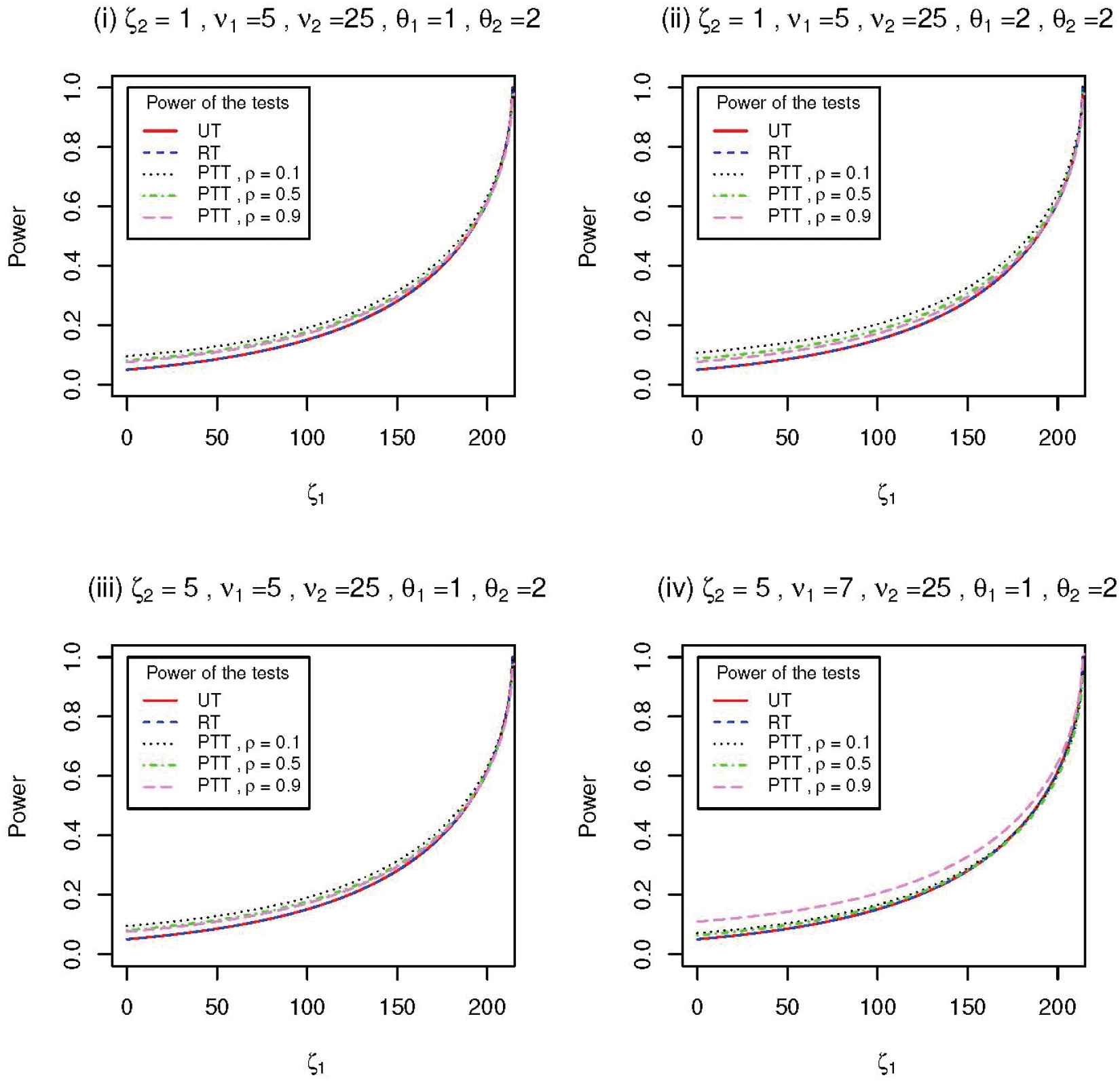
The power functions of the tests are computed for k=3, p=4, r=2, and s=2 so that δ1=β0,β1, δ2=β2,β3, and α1=α2=α3=α=0.05. Thus to compute the power of the tests, we fix the size to be 0.05 for all the tests. The power functions of the tests are calculated using the formulas in (27), (28), and (30). Whereas the graphs for the size of the three tests are produced using formulas in (34), (35), and (37). The power and size curves of the tests are shown in Figs. 1 and 2.
Figure 1
Comparing power of three tests against ζ1 with selected values of ρ, ζ2, df, and noncentrality parameters.
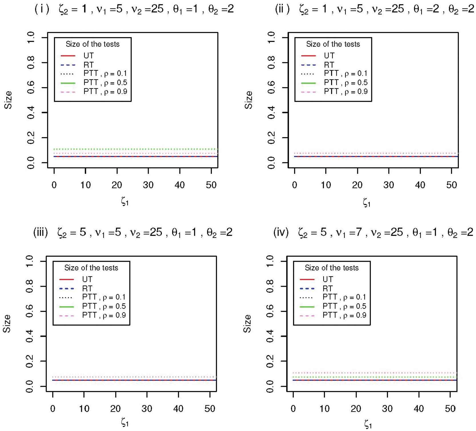
Figure 2
Comparison of size of three tests against ζ1 for selected values of ρ, ζ2, df, and noncentrality parameters.
8. POWER AND SIZE COMPARISON
Figure 1 shows that the power of the UT does not depend on ζ2 and ρ, but it slowly increases as the value of ζ1 increases. The form of the power curve of the UT is concave. For very small values of ζ1, near 0, the power curve of the UT slowly increases as ζ1 becomes larger. The power of the UT reaches its minimum, around 0.05, for ζ1=0 and for any value of ζ2.
Like the power of the UT, the power of the RT increases as the values of ζ1 increases and reaches 1 for large values of ζ1 (see Fig. 1). The power of the RT is greater, or equal to, than that of the UT for all values of ζ1 and/or ζ2. The RT achieves its minimum power, around 0.05, for ζ1=0 and all values of ζ2 (see Fig. 1). The maximum power of the RT is 1 for reasonably larger values of ζ1.
The power of the PTT depends on the values of ζ1, ζ2, and ρ. The power of the RT and PTT increases as the values of ζ1 and ζ2 increase for ρ=0.9. For ζ2=5 and ρ=0.9, the power of the PTT increases as the value of ν1 increases (see Fig. 1(d)), but not for ρ=0.1 and ρ=0.5. Moreover, the power of the PTT is always larger than that of the UT and tends to be the same as that of the RT for large values of ζ1 (see Fig. 1(d)). The minimum power of the PTT is around 0.07 for ζ1=0, and ρ=0.1,0.5 (see Fig. 1(d)), and it decreases (close to RT) as the value of ζ2 and ν1 becomes larger.
From Fig. 2 or (34) it is evident that the size of the UT does not depend on ζ2. It is constant for all values of ζ1 and ζ2. Like the size of the UT, the size of the RT is also constant for all values of ζ1 and ζ2. Moreover, the size of the RT is the same or larger than that of the UT for all values of ζ2 and does not depend on ρ.
The size of the PTT increases as the values of ν1 and ζ2 increase for ρ=0.9 (see Fig. 2(c) and 2(d)). But it decreases as the values of θ1 increases (see Fig. 2(a) and 2(b)).
The size of the UT is αUT=0.05 for all values of ζ1 and ζ2. The size of the RT, αRT≥αUT for all values of ζ2. The size of the PTT, αPTT≥αRT for all values of ζ1, a2 and ρ.
9. CONCLUSION
The above analyses reveal that the UT has lower power than the RT. The power of the UT is also less than that of the PTT for all values of ζ1 and ζ2 and ρ. The size of the RT and PTT is larger or equal to that of the UT for all values of ζ1 and ζ2.
For smaller values of ζ1, the UT and RT have lower power than the PTT. But for larger values of ζ1 the RT has higher, or same, power than the PTT and UT. Thus when the NSPI is reasonably accurate (i.e., ζ1 is small) the PTT over performs the UT and RT with higher power.
The UT has the smallest size among the three tests. But it also has the lowest power. The RT has the highest power and highest size. The PTT achieves higher power than the UT and lower size than the RT. Thus in the face of uncertainty, if NSPI is reasonably close to the true value of the parameters than the PTT is a better choice compared to UT and RT.
ACKNOWLEDGMENTS
The authors acknowledge valuable feedback of Emeritus Professor A K Md Ehsanes Saleh, Carleton University, Canada, and Dr Rossita M Yunus, University of Malaya, Malaysia for checking the computation of the power functions. The paper was completed when the first author visited Sultan Qaboos University, Oman.
REFERENCES
1.R. Mead, The Design of Experiments, Cambridge University Press, Cambridge, 1988, pp. 368.
2.K. Hinkelmann and O. Kempthorne, Design and Analysis of Experiments: Introduction to Experimental Design, Wiley, India, Vol. 1, 1994, pp. 350.
25.A.K.Md.E. Saleh and P.K. Sen, in Procedings of the Fifth Pannonian Symposium on Mathematical Statistics (Visegrád, Hungary), 13-18 September 1982, pp. 307-325.
26.R.M. Yunus and S. Khan, in 9th Islamic Countries Conference on Statistical Sciences (ICCS-IX): Statistics in the Contemporary World - Theories, Methods and Applications (Kuala Lumpur, Malaysia), 2007.
TY  - JOUR
AU  - Shahjahan Khan
AU  - Budi Pratikno
AU  - Shafiqur Rahman
AU  - M. Zakir Hossain
PY  - 2019
DA  - 2019/06/18
TI  - Tests on a Subset of Regression Parameters for Factorial Experimental Data with Uncertain Higher Order Interactions
JO  - Journal of Statistical Theory and Applications
SP  - 103
EP  - 112
VL  - 18
IS  - 2
SN  - 2214-1766
UR  - https://doi.org/10.2991/jsta.d.190514.001
DO  - 10.2991/jsta.d.190514.001
ID  - Khan2019
ER  -