
A New Generalized Two-Sided Class of the Distributions Via New Transmuted Two-Sided Bounded Distribution
- DOI
- 10.2991/jsta.d.190306.003How to use a DOI?
- Keywords
- Hazard rate function; order statistics; maximum likelihood estimator; transmutation map; transmuted two-sided distribution
- Abstract
In the present paper, we first consider a generalization of the standard two-sided power distribution so-called the transmuted two-sided distribution, and then extend proposed idea to generalized two-sided class of distributions, introduced by Korkmaz and Genç [1]. Some statistical and reliability properties including explicit expressions for quantiles, hazard rate function, order statistics, and maximum likelihood estimation are obtained in general setting. Generalized transmuted two-sided exponential distribution is considered as a especial case and denoted with the name
- Copyright
- © 2019 The Authors. Published by Atlantis Press SARL.
- Open Access
- This is an open access article distributed under the CC BY-NC 4.0 license (http://creativecommons.org/licenses/by-nc/4.0/).
1. INTRODUCTION
The statistical distribution theory has been widely explored by researchers in recent years. Given the fact that the data from our surrounding environment follow various statistical models, it is necessary to extract and develop appropriate high-quality models. One of the most important models in the statistical theory is the change point models. In the distribution theory, the change point distributions are used in the different branch of sciences such as economic, engineering, agriculture, and so on. Van Dorp and Kotz [2] introduced a family of the change point distributions so-called two-sided power (TSP) distribution with the probability density function (pdf),
The
One of the interesting methods for constructing new distributions is the transmutation map approach. Recently, some new distributions have been generalized based on the transmutation method. The transmuted distribution based on the
Aryal and Tsokos [12] generated a flexible family of probability distributions taking extreme value distribution as the base value distribution by using the quadratic rank transmutation map (QRTM). Aryal and Tsokos [13] generalized the two-parameter Weibull distribution using the QRTM. Aryal [14] introduced a generalization of the log-logistic distribution so-called the transmuted log-logistic distribution. Abd El Hady [15] introduced a new generalization of the two-parameter Weibull distribution by using the QRTM. This new distribution is named exponentiated transmuted Weibull (ETW) distribution. Elgarhy and Shawki [16] introduced a new generalized version of the quasi Lindley distribution which is called the transmuted generalized quasi Lindley (TGQL) distribution.
The transmutation method, as an important method for developing statistical distributions, hasn't been used for the change point distributions, yet. The main motivation of the present paper is to apply the transmutation technique for increasing the flexibility and usefulness of the
This paper organized as follows. In Section 2, we introduce a new distribution so-called transmuted two-sided distribution. In Section 3, we propose a generalization of the transmuted two-sided distribution and consider the hazard function, quantiles, and order statistics of this distribution. We consider the exponential distribution as a parent distribution and introduce transmuted two-sided generalized exponential (TSGE) distribution, in Section 4. In this section, we plot the shape of density function and hazard function. In Section 5, the estimation of parameters of the generalized transmuted two-sided distribution are obtained by using two methods maximum likelihood estimation (MLE) and bootstrap estimation. Also, we study the performance of MLEs of parameters of the transmuted TSGE distribution via a simulation study. In Section 6, the superiority of new model to some competitor statistical models is shown through the different criteria of selection model. Finally, the paper is concluded in Section 7.
2. TRANSMUTED TWO-SIDED DISTRIBUTION
In this section, we introduce the transmuted two-sided distribution and then we consider its shape for different values of parameters. The main motivation for introducing this new family is to provide the more flexibility for the
Let the random variable
Assume that
Using Eqs. (3) and (4) the
Now, suppose that
According to relations Eqs. (5) and (6), a new distribution is defined by
So, based on Eq. (7), we have the following definition.
Definition 2.1
A random variable
2.1. Density Shape of the TTS
Here, we consider a discussion about the shape of the proposed density function. In the end points of the support, the behaviour of the
The derivative
The right- and left-hand limits of
These limits are different. So,
When
When
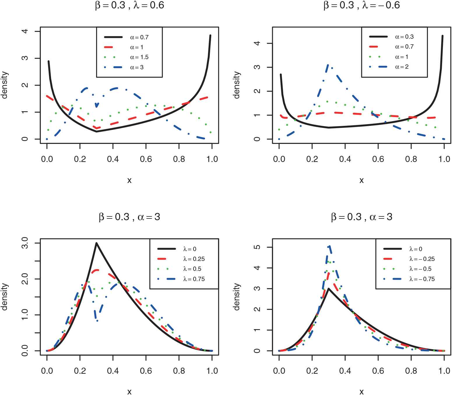
The graphs of the densities of the distribution.
3. TRANSMUTED TWO-SIDED GENERALIZED-G FAMILY OF THE DISTRIBUTIONS
Consider a continuous random variable with
Definition 3.1
A random variable
We denote transmuted TSG-G family of distributions by
Remark 3.1.
If
In the next subsections, we study hazard function, random variate generation, order statistics and relative entropy of the
3.1. Hazard Function
The hazard rate is a fundamental tools in reliability modelling for evaluation the ageing process. Knowing the shape of the hazard rate is important in reliability theory, risk analysis, and other disciplines. The concepts of increasing, decreasing, bathtub-shaped (first decreasing and then increasing) and upside-down bathtub-shaped (first increasing and then decreasing) hazard rate functions are very useful in reliability analysis. The lifetime distributions with these ageing properties are designated as the increasing failure rate (
3.2. Random Variate Generation
For generating random variables from the
Let
3.3. Order Statistics
Order statistics play a vital role in the theory of probability and statistics. Let
3.4. Kullback–-Leibler Divergence
The Kullback–Leibler divergence (or relative entropy) is an informational measure for comparing the similarity between two pdfs. The Kullback–Leibler divergence between the proposed distribution
On the other hand, if
The Shannon entropy of transmuted uniform distribution is computed by
From the relations, Eqs. (10) and (11) we see that the Kullback–Leibler divergence between the
4. TRANSMUTED TSGE DISTRIBUTION
The
We call this distribution the transmuted TSGE distribution and denote by
Remark 3.1.
If
4.1. Density Shape of the TTSG — E Distribution
In the end points of the support, the behaviour of the
The derivative
The right- and left-hand limits of
These limits are not equal. So,
In the next section, we consider the hazard shape of the
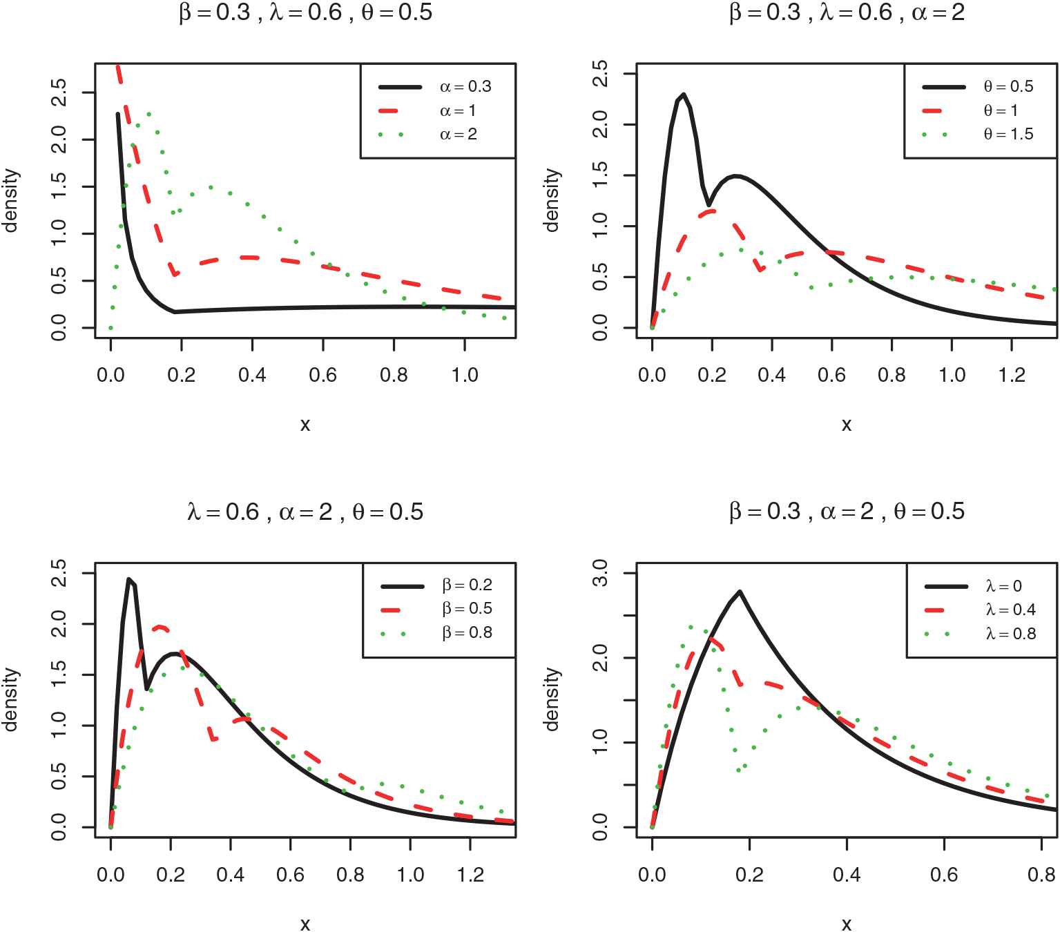
The graphs of the densities of the
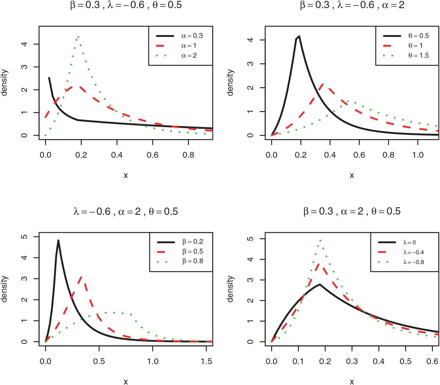
The graphs of the densities of the
4.2. Hazard Function of the TTSG — E Distribution
The hazard function of the
Because of complicated form of the hazard function, we couldn't explore this function analytically. We only consider the end points of the support. The behaviour of the hazard function in the end points is given as follows:
Some shapes of the hazard function for the selected values of parameters is given in Figs. 4 and 5. Figures 4 and 5 show that the hazard rate function of the
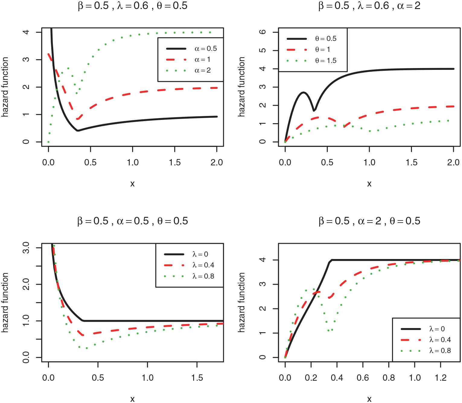
The graphs of the hazard function of the
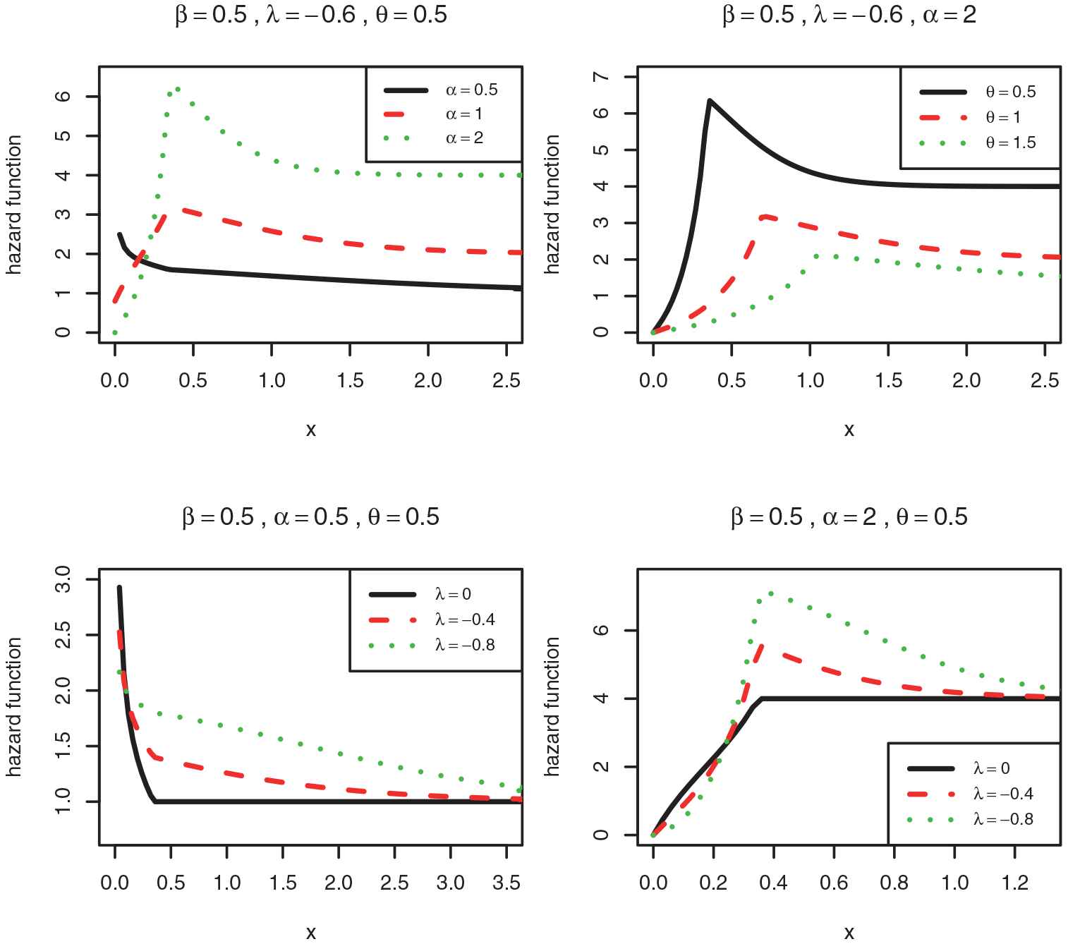
The graphs of the hazard function of the
5. ESTIMATION OF THE PARAMETERS OF THE TTSG — G DISTRIBUTION
In this section, we obtain the estimation of parameters the
5.1. Maximum Likelihood Estimation
Let
For estimating the parameters, we obtain the partial derivatives of the log-likelihood function with respect to the parameters. At the corner point
According to Van Dorp and Kotz [2] and Korkmaz and Genç [1], the
By taking the derivative of the log-likelihood function with respect to parameter vector
However, these equations are nonlinear and there are no explicit solutions. Thus, they have to be solved numerically. So, the
5.2. Bootstrap Estimation
The parameters of the fitted distribution can be estimated by parametric (resampling from the fitted distribution) bootstrap resampling (see Efron and Tibshirani [17]). The parametric bootstrap procedure is described as follows:
Parametric bootstrap procedure:
- 1
Estimate
- 2
Generate a bootstrap sample
- 3
Repeat Step 2
- 4
Order
In case of the
5.3. Simulation
Here, we assess the performance of the
| 30 | 0.0274 (0.0316) | 0.0165 (0.0099) | 0.0855 (0.0481) | 0.0272 (0.0229) | |
| 50 | 0.0153 (0.0269) | 0.0092 (0.0034) | 0.0721 (0.0502) | 0.0141 (0.0147) | |
| 100 | 0.0081 (0.0174) | 0.0045 (0.0030) | 0.0514 (0.0451) | 0.0063 (0.0071) | |
| 200 | 0.0035 (0.0098) | 0.0020 (0.0018) | 0.0243 (0.0245) | 0.0033 (0.0046) | |
| 30 | 0.0286 (0.0357) | 0.0181 (0.0093) | 0.0870 (0.0552) | 0.2462 (0.0742) | |
| 50 | 0.0156 (0.0294) | 0.0097 (0.0057) | 0.0720 (0.0552) | 0.1245 (0.0412) | |
| 100 | 0.0079 (0.0202) | 0.0042 (0.0011) | 0.0484 (0.0470) | 0.0632 (0.0352) | |
| 200 | 0.0035 (0.0097) | 0.0019 (−0.0007) | 0.0264 (0.0299) | 0.0285 (0.0138) | |
| 30 | 32.5268 (0.6036) | 0.0291 (0.0479) | 0.0914 (−0.0422) | 2.9212 (0.1673) | |
| 50 | 13.0018 (0.3243) | 0.0167 (0.0174) | 0.0449 (0.0192) | 1.1566 (0.0768) | |
| 100 | 0.1474 (0.0976) | 0.0063 (0.0019) | 0.0236 (0.0454) | 0.0132 (0.0142) | |
| 200 | 0.0412 (0.0524) | 0.0022 (−0.0016) | 0.0138 (0.0327) | 0.0025 (0.0072) | |
| 30 | 13.8834 (0.5349) | 0.0291 (0.0320) | 0.0946 (−0.0477) | 16.7689 (0.4470) | |
| 50 | 26.9195 (0.4725) | 0.0174 (0.0109) | 0.0460 (0.0255) | 12.5857 (0.3298) | |
| 100 | 2.0210 (0.1251) | 0.0067 (−0.0021) | 0.0249 (0.0396) | 1.5966 (0.0752) | |
| 200 | 0.0467 (0.0624) | 0.0023 (−0.0025) | 0.0150 (0.0388) | 0.0256 (0.0241) | |
| 30 | 16.0098 (0.6477) | 0.0589 (0.0013) | 0.8003 (0.8346) | 3.5771 (0.2223) | |
| 50 | 0.5018 (0.2976) | 0.0619 (0.0477) | 0.7082 (0.7889) | 0.2463 (0.0554) | |
| 100 | 0.2836 (0.2171) | 0.0600 (0.0730) | 0.4518 (0.6418) | 0.1114 (0.0304) | |
| 200 | 0.0460 (0.1789) | 0.0595 (0.0878) | 0.3221 (0.5549) | 0.0172 (0.0254) | |
| 30 | 5.7339 (0.5136) | 0.0664 (0.0481) | 0.8871 (0.8801) | 13.4951 (0.4215) | |
| 50 | 2.1495 (0.3433) | 0.0707 (0.0714) | 0.6986 (0.7841) | 8.0247 (0.2459) | |
| 100 | 0.0741 (0.2105) | 0.0666 (0.0826) | 0.4685 (0.6529) | 0.2054 (0.0803) | |
| 200 | 0.0449 (0.1787) | 0.0615 (0.0871) | 0.3225 (0.5558) | 0.1457 (0.0802) | |
| 30 | 83.3071 (3.0259) | 0.0518 (0.0820) | 0.8762 (0.8905) | 1.5715 (0.1644) | |
| 50 | 24.7184 (1.9937) | 0.0413 (0.0725) | 0.9042 (0.9040) | 0.4906 (0.0413) | |
| 100 | 4.6772 (1.5489) | 0.0344 (0.0633) | 0.9048 (0.9032) | 0.0876 (0.0049) | |
| 200 | 2.0712 (1.3450) | 0.0255 (0.0435) | 0.7545 (0.8364) | 0.0120 (−0.0076) |
MLE, maximum likelihood estimation; MSE, mean square error.
MSE and bias (values in parentheses) of the MLEs of the parameters α, β, λ, and θ.
6. APPLICATION OF THE TTSG — E DISTRIBUTION
To investigate the advantage of the proposed distribution, we consider a real data set provided by Bjerkedal [18]. This real data set consists of survival times of 72 guinea pigs injected with different amount of tubercle. This species of guinea pigs are known to have high susceptibility of human tuberculosis, which is one of the reasons for choosing. We consider only the study in which animals in a single cage are under the same regimen. The data represents the survival times of guinea pigs in days. The data are given below:
12 15 22 24 24 32 32 33 34 38 38 43 44 48 52 53 54 54 55 56 57 58 58 59 60 60 60 60 61 62 63 65 65 67 68 70 70 72 73 75 76 76 81 83 84 85 87 91 95 96 98 99 109 110 121 127 129 131 143 146 146 175 175 211 233 258 258 263 297 341 341 376.
6.1. Bootstrap Inference for Parameters of the TTSG — E Distribution
In this section, we obtain point and
| Point estimation | ||
|---|---|---|
| 2.223 | (1.354, 4.117) | |
| 0.298 | (0.157, 0.505) | |
| −0.307 | (−0.846, 0.734) | |
| 161.075 | (111.722, 268.019) |
CI, confidence interval.
Parametric bootstrap point and interval estimation of the parameters α, β, λ, and θ.
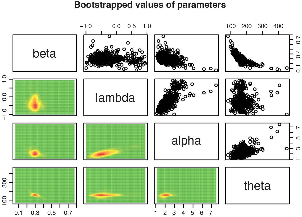
Parametric bootstrapped values of parameters of the TTSG — E distribution for the real data.
6.2. MLE
We fit the proposed distribution to the real data set by
For each model, Table 3 includes the
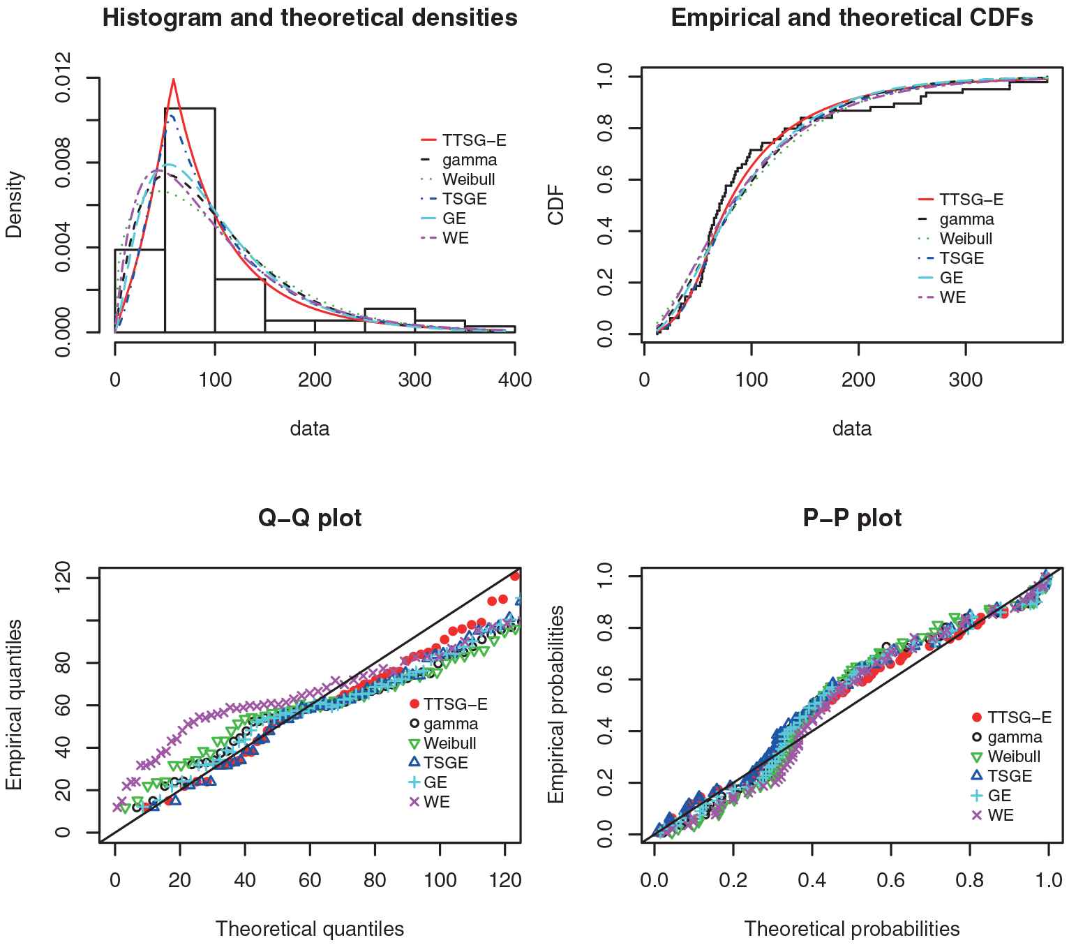
Histogram and fitted density plots, the plots of empirical and fitted
| Model | Estimation | Log-likelihood | |||
|---|---|---|---|---|---|
| −388.063 | 784.127 | 0.097 | 0.508 | ||
| gamma | −394.247 | 792.495 | 0.138 | 0.127 | |
| Weibull | −397.147 | 798.295 | 0.146 | 0.091 | |
| TSGE | −389.549 | 785.099 | 0.130 | 0.171 | |
| WE | −393.568 | 791.138 | 0.117 | 0.274 | |
| GE | −393.110 | 790.220 | 0.133 | 0.159 |
AIC, Akaike information criterion; GE, generalized exponential; K -- S, Kolmogorov -- Smirnov; MLE, maximum likelihood estimation; TSGE, two-sided generalized exponential, WE, weighted exponential.
The MLEs of parameters for real data set.
6.3. Likelihood Ratio Test
We use the likelihood ratio test
According to the LRT, the test statistic is given by
7. CONCLUDING REMARKS
In this paper, we propose a new family of distributions that is a compounding of two-sided distributions family and transmuted technique. The proposed model generalizes TSP distribution and generalized two-sided family of distributions and contains these distributions as its submodels. Some reliability and statistical properties of the proposed family of distribution are discussed through the paper. Estimation and inference procedure for distribution parameters are investigated by two well-known maximum likelihood and bootstrap methods in general setting. The
ACKNOWLEDGMENTS
The authors would like to thank the associate editor and referees for their constructive comments that improved presentation of the paper.
REFERENCES
Cite this article
TY  - JOUR
AU  - O. Kharazmi
AU  - M. Zargar
PY  - 2019
DA  - 2019/06/18
TI  - A New Generalized Two-Sided Class of the Distributions Via New Transmuted Two-Sided Bounded Distribution
JO  - Journal of Statistical Theory and Applications
SP  - 87
EP  - 102
VL  - 18
IS  - 2
SN  - 2214-1766
UR  - https://doi.org/10.2991/jsta.d.190306.003
DO  - 10.2991/jsta.d.190306.003
ID  - Kharazmi2019
ER  -