
Statistical Properties and Different Estimation Procedures of Poisson–Lindley Distribution

- DOI
- 10.2991/jsta.d.210105.001How to use a DOI?
- Keywords
- Anderson–Darling method; Cramer–von Mises; Least square estimators; Maximum likelihood estimators; Poisson–Lindley distribution
- Abstract
In this paper, we propose a new class of distributions by compounding Lindley distributed random variates with the number of variates being zero-truncated Poisson distribution. This model is called a compound zero-truncated Poisson–Lindley distribution with two parameters. Different statistical properties of the proposed model are discussed. We describe different methods of estimation for the unknown parameters involved in the model. These methods include maximum likelihood, least squares, weighted least squares, Cramer–von Mises, maximum product of spacings, Anderson–Darling and right-tail Anderson–Darling methods. Numerical simulation experiments are conducted to assess the performance of the so obtained estimators developed from these methods. Finally, the potentiality of the model is studied using one real data set representing the monthly highest snowfall during February 2018, for a subset of stations in the Global Historical Climatological Network of USA.
- Copyright
- © 2021 The Authors. Published by Atlantis Press B.V.
- Open Access
- This is an open access article distributed under the CC BY-NC 4.0 license (http://creativecommons.org/licenses/by-nc/4.0/).
1. INTRODUCTION
In recent years, many researches are interested in obtaining several new continuous distributions by compounding an absolutely continuous distribution with a discrete distribution. This method is used widely in engineering applications including risk measurement, floods reliability and survical analysis. For example, Adamidis and Loukas [1] proposed a two-parameter lifetime distribution by compounding exponential and geometric distributions. The exponential Poisson (EP) and exponential logarithmic distributions were introduced by Kus [2] and Tahmasbi and Rezaei [3], respectively. Marshall and Olkin [4] developed some new extensions based on random minimum and maximum. Barreto-Souza and Cribari-Neto [5] introduced the exponentiated exponential Poisson (EEP).
Cancho et al. [6] introduced the Poisson-exponential (PE) distribution by compounding the exponential and zero-truncated Poisson distributions. Chahkandi and Ganjali [7] introduced a class of distributions, namely exponential power series (EPS) distributions by compounding exponential and power series distributions. Also in the same way, Mahmoudi and Jafari [8] introduced the generalized exponential power series (GEPS) distribution by compounding the generalized exponential (GE) distribution with the power series distribution. The performances of the estimators using intensive simulation experiments have received considerable attention in the literature by several authors. Among them, Gupta and Kundu [9], Kundu and Raqab [10], Alkasabeh and Raqab [11], Asgharzadeh et al. [12], Dey et al. [13] and Rodrigues et al. [14].
The main aim of the present study is two-fold. The first main aim is to introduce a new model which is flexible in fitting a wide range of data sets by compounding Lindley and zero-truncated Poisson distributions. The basic idea can be described as follows. Consider a random variable
Given
Here, we introduce a new class of distributions based on the maximal random variate
The second aim is to present various estimation methods for estimating the two parameters of the compound ZTPL model. The estimators to be considered are maximum likelihood estimators (MLEs), least square estimators (LSEs), weighted least square estimators (WLSEs), Cramer–von Mises type minimum distance estimators (CMDEs), maximum product of spacings, Anderson–Darling estimators (ADEs) and right-tail Anderson–Darling estimation (RTADE). An intensive simulation study is performed for comparing the effectiveness of the so developed of estimators.
This paper is organized as follows: In Section 2, the ZTPL model is described and its distributional properties are discussed. Also, different methods for estimating the parameters of the ZTPL model are developed in Section 3. Numerical simulation results are presented in Section 4. The analysis of monthly highest snowfall data during the month of February 2018, for a subset of stations in the Global Historical Climatological Network of USA is performed for validation purposes in Section 5. Some concluding remarks are presented in Section 6.
2. ZTPL DISTRIBUTION
A random variable
The corresponding PDF of
From (6), it is easily seen that the Lindley distribution is a special case of compound ZTPL when
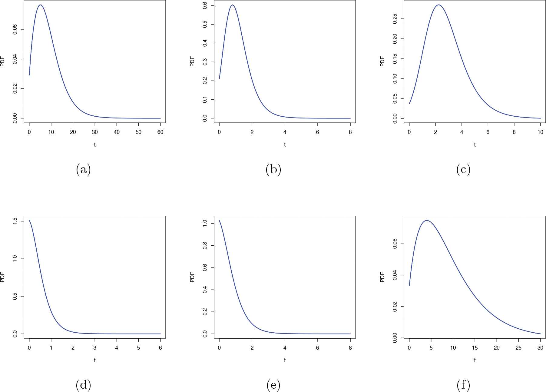
Probability density function (PDF) plots of zero-truncated Poisson–Lindley (ZTPL) distribution for different parameter values: (a) (0.25, 1) (b) (2, 3) (c) (1, 4) (d) (3, 0.75) (e) (2, 0.5) (f) (0.2, 0.0001).
The joint PDF of
Further, from (6) and (7), it can be shown that the PDF of the conditional distribution of
The survival function and hazard rate (HR) of the
Figure 2 presents different shapes of HR for the compound ZTPL(
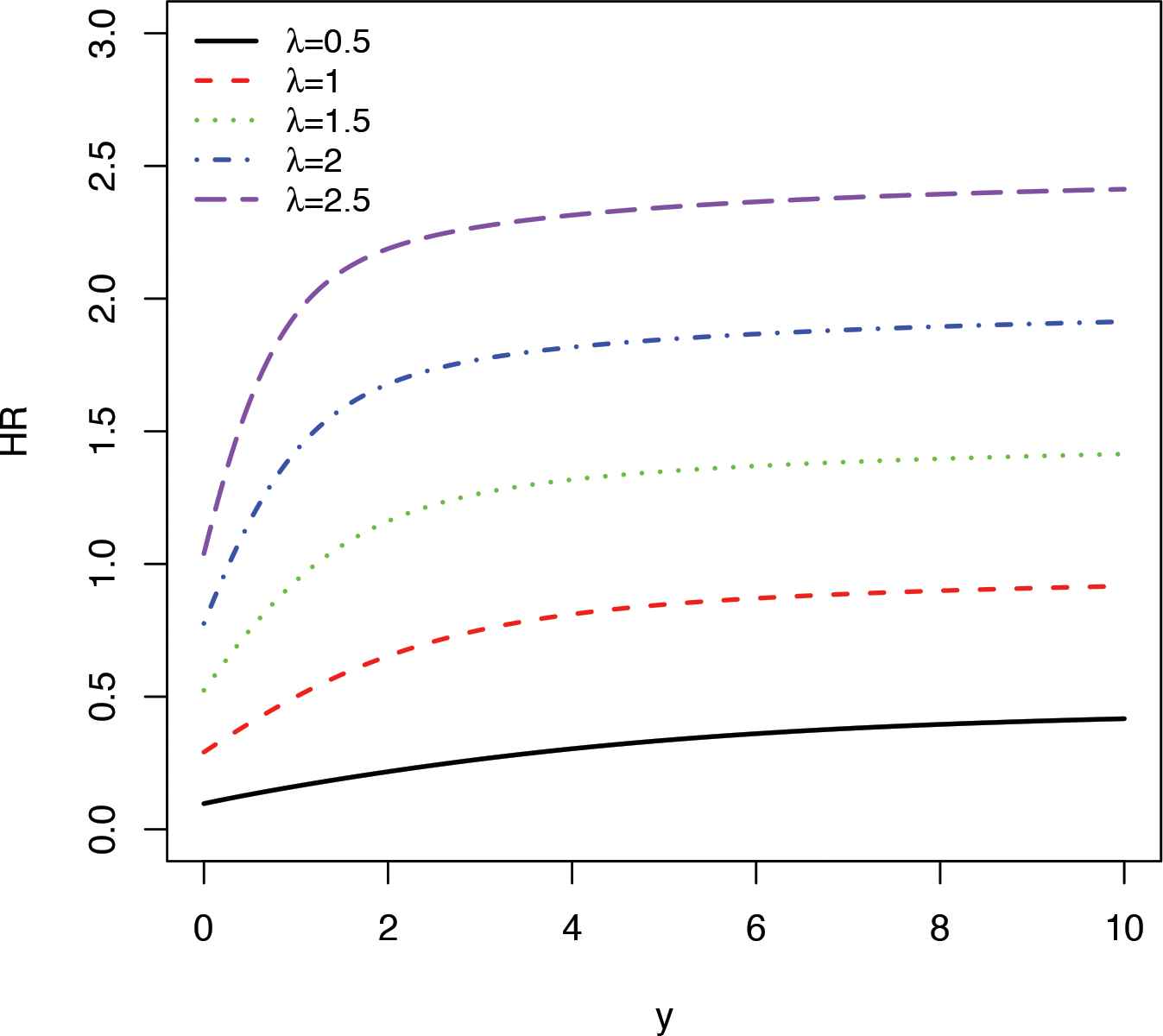
HR Plots for λ = 0.5, 1, 1.5, 2, 2.5 and fxed θ = 1.
The following expression for the
Therefore, the mean and variance of
The skewness measure of
The moment generating function (MGF) of
3. METHODS OF ESTIMATION
In this section, we present different estimation methods for obtaining the estimators of the parameters
3.1. Maximum Likelihood Estimation and its Asymptotics
Let
The MLEs
Another aspect of estimation is to construct confidence intervals (CIs) of the parameters by making use of the asymptotic distribution theory of MLE. By denoting the parameter vector
The elements of matrix
Therefore, the lower confidence limit (LCL) and upper confidence limit (UCL) of
Then the
3.2. Least Square and Weighted LSEs
Swain et al. [15] proposed an alternative method to compute the estimation of unknown parameters, which is called the LSEs or WLSEs. The basic idea can be defined as follows. Let
The WLSEs of
Hence, the estimates
3.3. Maximum Product of Spacings
Cheng and Amin [16,17] introduced an elaborate technique to compute the estimation of unknown parameters of continuous univariate distributions, namely the maximum product spacing (MPS) method. It was developed by Ranneby [18] independently as an approximation to the Kullback–Leibler measure of information. The simple idea can be described as follows. Let
Clearly
The MPS estimators (MPSEs) of
Equivalently, they can be obtained by maximizing the logarithm of the geometric mean of sample spacings:
The estimates
3.4. Cramer–von Mises Minimum Distance Estimators
The CMDEs can be obtained as the difference between the estimate of the CDF and its respective empirical distribution function. MacDonald [19] provided empirical evidence that the bias of the estimator is smaller than the other minimum distance estimators. The Cramer–von Mises estimates
These estimates can also be obtained by solving the nonlinear equations:
3.5. Anderson–Darling and Right-Tail Anderson–Darling
The ADE is another type of minimum distance estimator and it was introduced by Anderson and Darling [20]. The ADEs
These estimates can also be obtained by solving the following equations:
Similarly, the RTADEs,
These estimates can be obtained by solving the the following equations:
4. NUMERICAL EXPERIMENTS AND DISCUSSIONS
In this section, we present some results of Monte Carlo simulation study to compare the efficiency of the different estimation procedures proposed in the previous sections. For a given set of parameter values for
| Par | Est. | MLE | LSE | WLSE | CME | MPS | ADE | RTADE | |
|---|---|---|---|---|---|---|---|---|---|
| 25 | AE | 0.5673 | 0.4897 | 0.4929 | 0.5263 | 0.4816 | 0.5102 | 0.4686 | |
| MSE | 0.0200 | 0.0316 | 0.0315 | 0.0313 | 0.0041 | 0.0257 | 0.0218 | ||
| 50 | AE | 0.5437 | 0.4829 | 0.4802 | 0.5040 | 0.4983 | 0.4975 | 0.4902 | |
| MSE | 0.0089 | 0.0170 | 0.0146 | 0.0158 | 0.0024 | 0.0175 | 0.0113 | ||
| 100 | AE | 0.5227 | 0.4873 | 0.5003 | 0.4997 | 0.4992 | 0.4914 | 0.5027 | |
| MSE | 0.0042 | 0.0096 | 0.0067 | 0.0084 | 0.0011 | 0.0046 | 0.0064 | ||
| 300 | AE | 0.5098 | 0.4891 | 0.4990 | 0.4986 | 0.5004 | 0.4942 | 0.5050 | |
| MSE | 0.0015 | 0.0036 | 0.0020 | 0.0028 | 0.0009 | 0.0020 | 0.0023 | ||
| 500 | AE | 0.5026 | 0.5049 | 0.4968 | 0.5007 | 0.5090 | 0.5008 | 0.5022 | |
| MSE | 0.0010 | 0.0014 | 0.0013 | 0.0016 | 0.0003 | 0.0013 | 0.0010 | ||
| 25 | AE | 1.1585 | 0.2207 | 0.1742 | 0.6038 | 0.4670 | 0.4126 | 0.1417 | |
| MSE | 1.6850 | 2.6828 | 3.2857 | 3.2989 | 0.0076 | 2.7555 | 3.8645 | ||
| 50 | AE | 0.8743 | 0.2743 | 0.2389 | 0.4794 | 0.4896 | 0.4011 | 0.3443 | |
| MSE | 0.8223 | 2.4417 | 1.7143 | 1.6978 | 0.0010 | 1.9692 | 1.4611 | ||
| 100 | AE | 0.5960 | 0.3460 | 0.4395 | 0.4713 | 0.4963 | 0.4337 | 0.4771 | |
| MSE | 0.3872 | 0.9877 | 0.7283 | 0.9177 | 0.0008 | 0.5503 | 0.8661 | ||
| 300 | AE | 0.3400 | 0.4181 | 0.4931 | 0.4756 | 0.5049 | 0.4486 | 0.5061 | |
| MSE | 0.1264 | 0.3812 | 0.2301 | 0.2816 | 0.0007 | 0.2131 | 0.2165 | ||
| 500 | AE | 0.5292 | 0.5073 | 0.4734 | 0.5011 | 0.5097 | 0.4915 | 0.5216 | |
| MSE | 0.0960 | 0.1335 | 0.1338 | 0.1657 | 0.0003 | 0.1373 | 0.0969 |
AE, average estimate; MSE, mean squared error; MLE, maximum likelihood estimator; LSE, least square estimator; WLSE, weighted least square estimator; MPS, maximum product spacing; ADE, Anderson–Darling estimator; RTADE, right-tail Anderson–Darling estimator.
The AE and the associated MSEs for the estimates of
| Par | Est. | MLE | LSE | WLSE | CME | MPS | ADE | RTADE | |
|---|---|---|---|---|---|---|---|---|---|
| 25 | AE | 1.0759 | 0.9318 | 0.9798 | 1.0336 | 0.9598 | 0.9866 | 1.0077 | |
| MSE | 0.0508 | 0.1168 | 0.0937 | 0.0938 | 0.0202 | 0.0864 | 0.0954 | ||
| 50 | AE | 1.0092 | 0.9861 | 0.9562 | 1.0146 | 0.9808 | 0.9430 | 1.0216 | |
| MSE | 0.0207 | 0.0601 | 0.0437 | 0.0565 | 0.0084 | 0.0446 | 0.0477 | ||
| 100 | AE | 1.0223 | 0.9873 | 1.0170 | 1.0215 | 0.9912 | 0.9958 | 1.0153 | |
| MSE | 0.0143 | 0.0351 | 0.0220 | 0.0262 | 0.0030 | 0.0244 | 0.0248 | ||
| 300 | AE | 1.0015 | 0.9865 | 0.9780 | 1.0080 | 1.0056 | 1.0096 | 0.9913 | |
| MSE | 0.0048 | 0.0098 | 0.0082 | 0.0086 | 0.0026 | 0.0085 | 0.0070 | ||
| 500 | AE | 1.0034 | 1.0043 | 1.0053 | 1.0014 | 1.0176 | 1.0025 | 1.0078 | |
| MSE | 0.0037 | 0.0049 | 0.0044 | 0.0047 | 0.0020 | 0.0044 | 0.0034 | ||
| 25 | AE | 1.0774 | 0.2428 | 0.5457 | 0.8378 | 0.7257 | 0.4698 | 0.7177 | |
| MSE | 1.2320 | 3.6427 | 2.4906 | 2.2156 | 0.0071 | 2.8561 | 3.0602 | ||
| 50 | AE | 0.8486 | 0.6438 | 0.5907 | 0.7168 | 0.7453 | 0.4715 | 0.8298 | |
| MSE | 0.5147 | 1.7936 | 1.2246 | 1.1642 | 0.0012 | 1.3342 | 1.3694 | ||
| 100 | AE | 0.8745 | 0.6277 | 0.8020 | 0.8503 | 0.7480 | 0.6720 | 0.8176 | |
| MSE | 0.4271 | 0.8848 | 0.5889 | 0.5837 | 0.0008 | 0.6024 | 0.6815 | ||
| 300 | AE | 0.7589 | 0.6678 | 0.6496 | 0.7904 | 0.7520 | 0.7519 | 0.7044 | |
| MSE | 0.1057 | 0.2395 | 0.1890 | 0.1721 | 0.0006 | 0.1865 | 0.1870 | ||
| 500 | AE | 0.7682 | 0.7524 | 0.7613 | 0.7523 | 0.7583 | 0.7775 | 0.8085 | |
| MSE | 0.1000 | 0.1024 | 0.1045 | 0.1041 | 0.0005 | 0.1090 | 0.0978 |
AE, average estimate; MSE, mean squared error; MLE, maximum likelihood estimator; LSE, least square estimator; WLSE, weighted least square estimator; MPS, maximum product spacing; ADE, Anderson–Darling estimator; RTADE, right-tail Anderson–Darling estimator.
The AE and the associated MSEs for the estimates of
Some of the points are quite clear from Tables 1 and 2. As the sample size increases, the AEs based on all estimation methods tend to the true parameter values and the MSEs decrease. This indicates that all estimators are consistent and asymptotically unbiased. Furthermore, it is observed that as
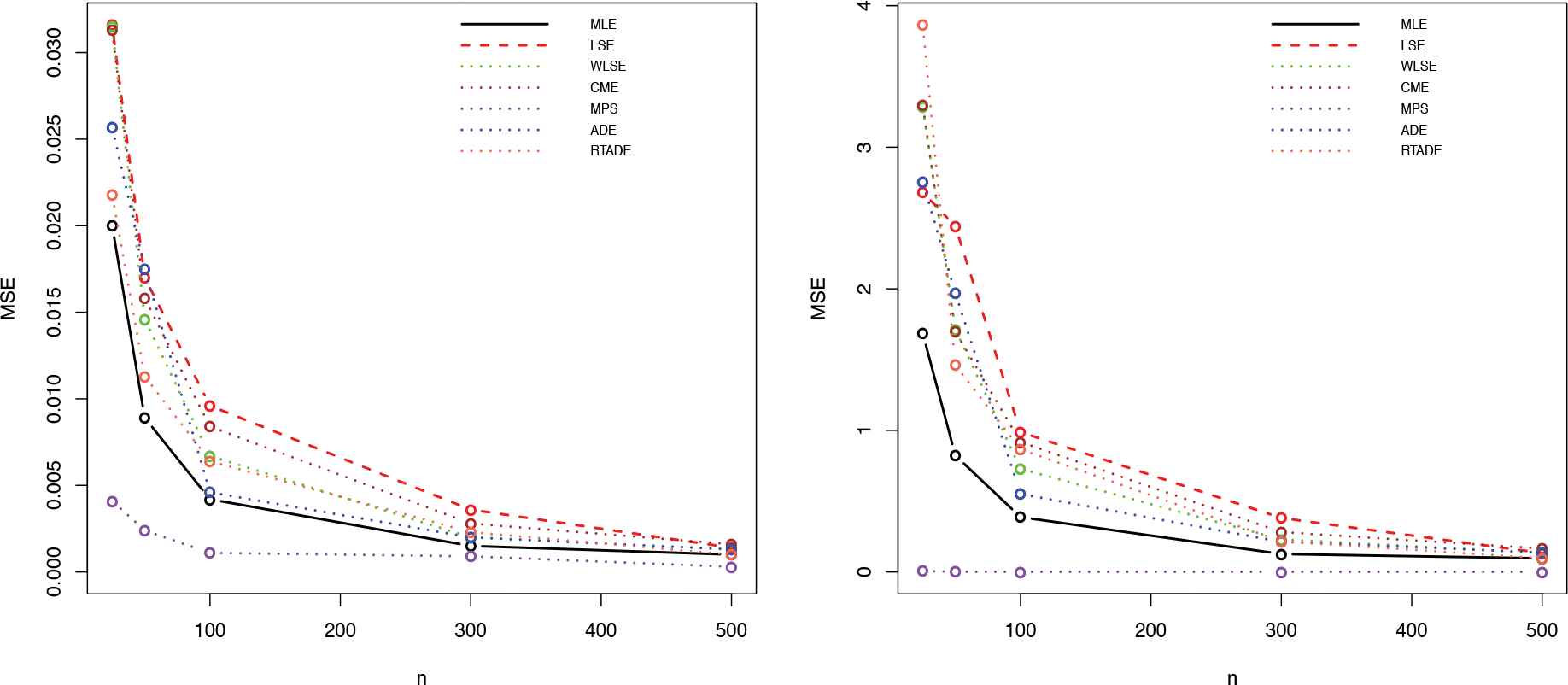
MSE of
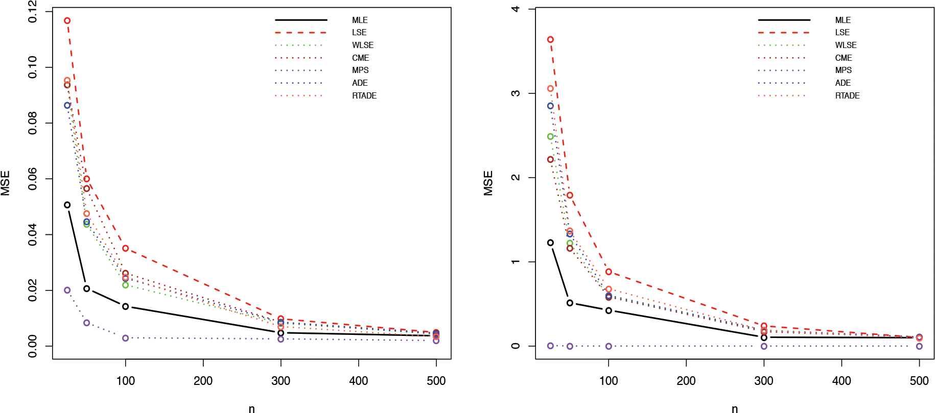
MSE of
5. APPLICATION TO MONTHLY MAXIMUM SNOWFALL DATA
In this section, we discuss the analysis of real-life data representing the monthly highest snowfall during the month of February 2018, obtained from a subset of stations in the United States and it is measured in inches (in). This data set was reported in: the National Centers for Environmental Information (NCEI) (https://www.ncdc.noaa.gov/cdoweb/datatools/records). Here, we only wish to demonstrate the use of the estimation procedures based on samples from compound ZTPL model. Table 3 summarizes some basic statistics of the monthly maximum snowfall data set.
| Mean | Median | Std.Dev. | ||
|---|---|---|---|---|
| 8.25 | 7.99 | 3.50 | 5.98 | 10.09 |
Basic statistics of monthly highest snowfall data set.
The following distributions are used in the literature as fitting models for the data set. For example, Poisson Lomax PL
| Distribution | Parameters | ll |
|---|---|---|
| Lindley | −156.4475 | |
| ZTPL | −143.1997 | |
| PL | −145.3201 | |
| EWP | −152.0237 |
MLE, maximum likelihood estimator; ZTPL, zero-truncated Poisson–Lindley; EWP, exponentiated Weibull–Poisson.
The MLEs and the corresponding log-likelihood (ll) values for different fitting distributions.
For further checking model validity and comparisons, the values of K-S and other criteria and their corresponding p values for other distributions including Lindley, PL and EWP distributions are computed. The additional considered criteria are Akaike information criterion (AIC), Akaike information criterion correction (AICc), Hannan–Quinn information criterion (HQIC), Bayesian information criterion (BIC). Table 5 presents the values of these statistics. Note that the smaller the value of the considered criterion, the better the fit to the data. Clearly, the compound ZTPL distribution is a good alternative model comparing with other fitted models. Figure 5 shows the plots of the fitted PDFs and CDFs with their corresponding empirical values. In addition, the empirical survival function (ESF) and fitted survival function are presented in Figure 6. All these plots confirm the same conclusion. Now, we obtain the estimators of the unknown parameters for the compound ZTPL model using different methods of estimation discussed in Section 3. The results for estimates as well as LCL and UCL for
| Distribution | AIC | AICc | HQIC | BIC | K-S | |
|---|---|---|---|---|---|---|
| Lindley | 314.8949 | 314.9719 | 315.6620 | 316.8839 | 0.2398 | 0.004 |
| ZTPL | 290.3994 | 290.6347 | 291.9335 | 294.3774 | 0.1109 | 0.5197 |
| PL | 296.6401 | 297.1201 | 298.9414 | 302.6071 | 0.1267 | 0.3512 |
| EWP | 312.0474 | 312.8637 | 315.1156 | 320.0033 | 0.1587 | 0.1317 |
MLE, maximum likelihood estimator; ZTPL, zero-truncated Poisson–Lindley; EWP, exponentiated Weibull–Poisson; AIC, Akaike information criterion; AICc, Akaike information criterion correction (AICc); HQIC, Hannan–Quinn information criterion; BIC, Bayesian information criterion; K-S, Kolmogorov–Smirnov.
The goodness of fit tests for monthly highest snowfall data set.
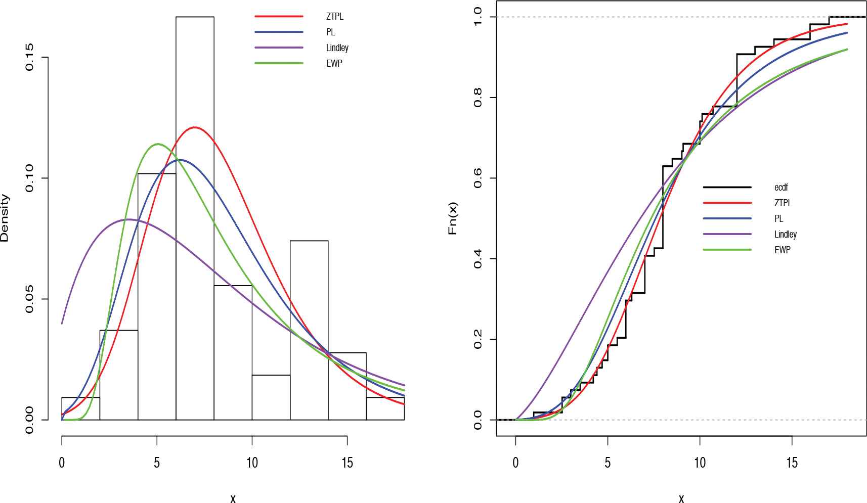
Fitted and empirical densities and cumulative distribution functions (CDFs) of zero-truncated Poisson–Lindley (ZTPL), PL, Lindley and exponentiated Weibull–-Poisson (EWP) distributions for the monthly highest snowfall data set.
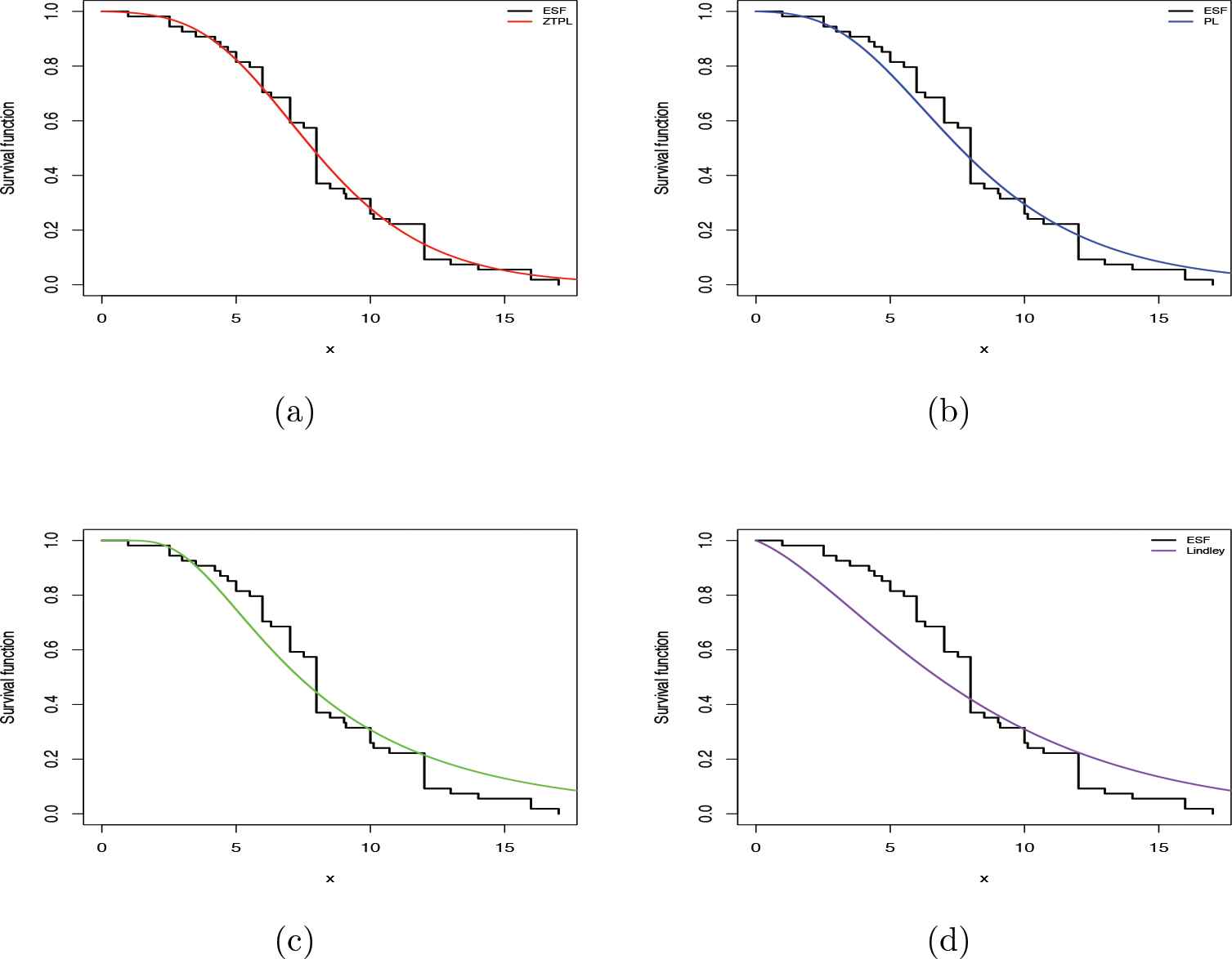
The empirical survival function (ESF) and fitted survival functions for different distributions: (a) zero-truncated Poisson–Lindley (ZTPL), (b) PL, (c) exponentiated Weibull–-Poisson (EWP) and (d) Lindley.
| Method | ll | K-S | ||||||
|---|---|---|---|---|---|---|---|---|
| Est. | LCB | UCB | Est. | LCB | UCB | |||
| MLE | 0.4258 | 0.3471 | 0.5078 | 5.8033 | 4.1696 | 7.4369 | −143.1997 | 0.1109 |
| LSE | 0.4309 | 0.3477 | 0.5140 | 6.1238 | 4.4186 | 7.8289 | −143.2309 | 0.1173 |
| WLSE | 0.4239 | 0.3421 | 0.5056 | 5.8177 | 4.1809 | 7.4544 | −143.2049 | 0.1165 |
| CME | 0.4423 | 0.3569 | 0.5276 | 6.6075 | 4.7906 | 8.4243 | −143.3629 | 0.1162 |
| MPS | 0.4341 | 0.3503 | 0.5178 | 5.8224 | 4.1845 | 7.4602 | −143.1989 | 0.1104 |
| ADE | 0.4278 | 0.3453 | 0.5102 | 5.9683 | 4.2981 | 7.6384 | −143.2100 | 0.1160 |
| RTADE | 0.4383 | 0.3537 | 0.5228 | 6.4321 | 4.6562 | 8.2079 | −143.3023 | 0.1165 |
CI, confidence interval; MSE, mean squared error; MLE, maximum likelihood estimator; LSE, least square estimator; WLSE, weighted least square estimator; MPS, maximum product spacing; ADE, Anderson–Darling estimator; RTADE, right-tail Anderson–Darling estimator.
Estimates of
6. CONCLUSION
In this paper, a new family of distributions is proposed based on a maxima of Poisson number of Lindely random variates. It is called a compound ZTPL model. Some distributional properties of this model are discussed and different methods of estimation are derived for the unknown parameters, namely, maximum likelihood, least squares, weighted least squares, Cramer–von Mises, maximum product of spacing, Anderson–Darling and right tailed Anderson–Darling. It is observed that the estimators obtained by maximum product of spacing method outperform all other estimators when the mean square error is considered as an optimality criterion. For fitting the maximal values of random number observations, it is evident that the compound ZTPL model provides a consistently better fit than Lindley, Poisson Lomax and Exponentiated Weibul–Poisson distributions.
CONFLICTS OF INTEREST
The authors have no conflicts of interests to declare.
Funding Statement
No funding
ACKNOWLEDGEMENTS
Thanks are due to referees’ comments that helped to improve the paper
REFERENCES
Cite this article
TY  - JOUR
AU  - Mohammed Amine Meraou
AU  - Mohammad Z. Raqab
PY  - 2021
DA  - 2021/01/11
TI  - Statistical Properties and Different Estimation Procedures of Poisson–Lindley Distribution
JO  - Journal of Statistical Theory and Applications
SP  - 33
EP  - 45
VL  - 20
IS  - 1
SN  - 2214-1766
UR  - https://doi.org/10.2991/jsta.d.210105.001
DO  - 10.2991/jsta.d.210105.001
ID  - Meraou2021
ER  -